The Dimension Dilemma: Why 2.5D Models Outperform 3D CNNs for Stroke Classification
Lessons & Experiments on training deep learning models on 3D medical data.
Introduction: A Surprising Discovery
When I started this project, I was convinced that 3D convolutional neural networks were the obvious choice for analyzing brain CT scans. After all, the brain is inherently a 3D structure, and 3D CNNs can capture volumetric spatial relationships that 2D slice-by-slice approaches might miss. The literature seemed to confirm this intuition—paper after paper touted the superiority of 3D models for medical imaging tasks.
Two months later, after training dozens of models and debugging countless experiments, I learned a humbling lesson: sometimes the theoretically superior approach fails in practice, and the "simpler" solution wins.
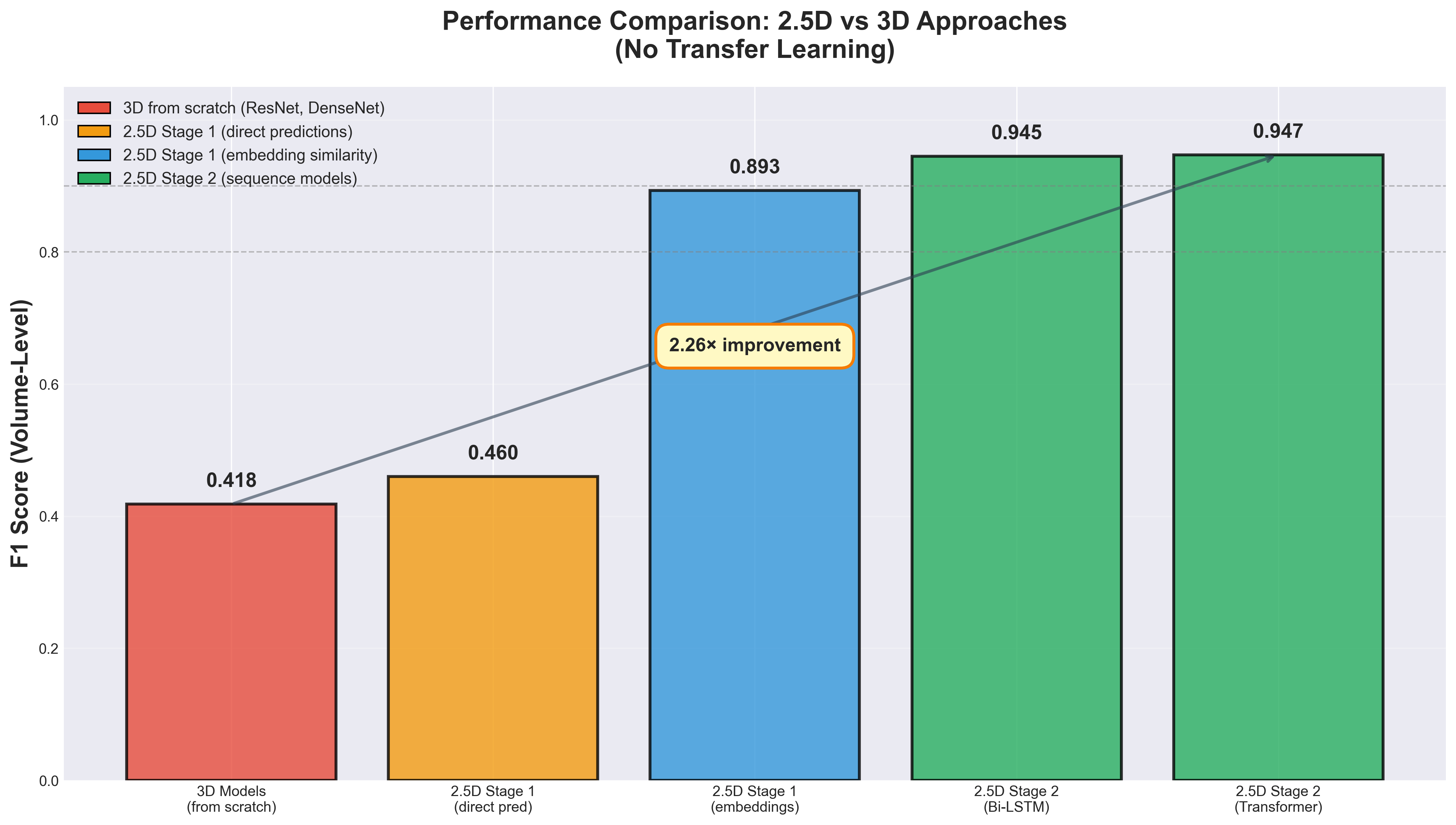
Here's the punchline: A 2.5D model combining a 2D CNN with an LSTM sequence model achieved an F1 score of 0.945 on volume-level stroke classification, while my best 3D model topped out at F1 = 0.418. The gap wasn't marginal; it was catastrophic and consistent across multiple architectures and training configurations.
This blog post chronicles that experimental journey from failure to success, presenting quantitative results and practical insights for anyone working with volumetric medical data. If you're debating whether to use 2D, 2.5D, or 3D architectures for your next medical imaging project, this post is for you.
The Task: Stroke Classification from CT Scans
Before diving into model architectures, let's establish the problem we're trying to solve.
Why Stroke Classification Matters
Stroke is the second leading cause of death globally, and one in four adults over age 25 will experience a stroke in their lifetime. More critically, the type of stroke determines the treatment. Ischemic strokes, which account for 87% of cases, are caused by blood vessel blockage and may benefit from clot-dissolving medications. Hemorrhagic strokes, comprising 13% of cases, result from ruptured vessels causing bleeding in the brain.
Administering thrombolytic drugs to an ischemic stroke patient can save brain tissue. Giving the same treatment to a hemorrhagic stroke patient could be fatal, as it would exacerbate bleeding. Rapid and accurate diagnosis is literally life-or-death.
The Data
I worked with three publicly available datasets for this research. The RSNA 2019 Brain CT Hemorrhage Challenge dataset provided over 25,000 scans with five hemorrhage subtypes plus control cases, totaling more than 700,000 individual slices. This dataset became my primary focus due to its size and inclusion of healthy control scans, enabling true classification rather than just detection. The AISD dataset contributed 397 ischemic stroke scans with paired CT-MRI images and manual lesion contours. The CPAISD dataset offered 112 acute ischemic stroke scans with penumbra and core delineation, all captured within 24 hours of symptom onset.
| Dataset | Size | Stroke Type | Key Features | Link |
|---|---|---|---|---|
| RSNA 2019 | 25,000+ scans | Hemorrhagic + Control | 5 hemorrhage subtypes 700,000+ slices | Kaggle |
| AISD | 397 scans | Ischemic (acute) | Paired NCCT-MRI Manual lesion contours | GitHub |
| CPAISD | 112 scans | Ischemic (acute) | Penumbra & core delineation Within 24h of symptoms | Zenodo |
Preprocessing: From DICOM to Model Input
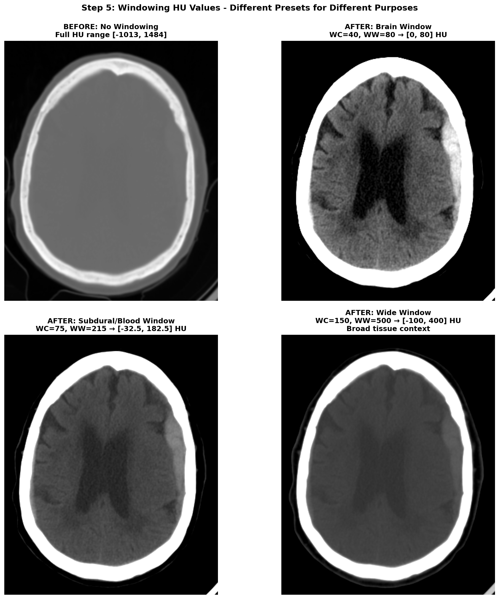
CT images require careful preprocessing before feeding into deep learning models. The process begins with Hounsfield Unit (HU) conversion, transforming raw DICOM pixel values into a standardized tissue density scale where water equals 0, air equals -1000, and dense bone reaches +1000. Next comes volume reconstruction, where slices must be correctly ordered along the z-axis —getting this wrong can scramble the anatomical sequence. Resampling standardizes voxel spacing to consistent resolution across different scanners and acquisition protocols. Brain cropping removes the skull, scalp, and scanner artifacts that add noise without contributing to stroke detection. Windowing restricts the HU range to highlight relevant anatomy; different window settings emphasize different tissue types, as shown in Figure 1 below. Finally, data augmentation through horizontal flips, small rotations, and intensity variations helps the model generalize beyond the training distribution.
For readers interested in a detailed explanation of each preprocessing step, I've written a companion blog post dedicated to processing CT images for stroke detection.
The Challenge
CT brain volumes are high-dimensional by nature. A typical scan contains 15-60 slices, each with resolution of 512×512 pixels. After preprocessing and downsampling to manageable sizes like 128×128, a volume might still be 64×128×128 voxels—a hefty input for 3D CNNs. With limited data, despite RSNA being relatively large by medical imaging standards, and these massive input dimensions, training deep 3D models from scratch is notoriously difficult. But I was determined to make it work.
The Seductive Promise of 3D Models
Why did I believe 3D models were the answer? The reasoning seemed airtight.
Theoretical Advantages of 3D CNNs
First, 3D convolutions provide native volumetric reasoning, naturally capturing spatial relationships across all three dimensions simultaneously rather than treating slices independently. Second, anatomical context matters profoundly—the brain is a 3D organ where pathology location carries diagnostic significance, as a hemorrhage in the subdural space differs fundamentally from one in the parenchyma. Third, stroke lesions often span multiple consecutive slices, creating 3D patterns that emerge only when viewing the full volume rather than individual slices. Fourth, the literature offered strong support, with multiple papers reporting superior performance of 3D models over 2D approaches for medical imaging tasks.
What the Literature Suggested
The research literature on brain imaging consistently showed 3D architectures outperforming 2D alternatives. For stroke detection specifically, several studies reported that 3D models could learn more discriminative features from volumetric context, better localize small lesions appearing on only a few slices, and achieve higher sensitivity and specificity than slice-wise approaches.
The papers that particularly influenced my initial approach explored multi-task learning frameworks combining classification and segmentation. Research by Huang et al. [1] demonstrated how dual-task models could leverage shared representations to improve both tasks simultaneously. Two other influential works [2, 3] showed promising results for similar medical imaging challenges using 3D architectures, reinforcing the intuition that volumetric processing should outperform 2D approaches. Additional studies [9, 10, 11] reported strong performance using 3D CNNs and vision transformers for stroke classification, further supporting the theoretical advantages of volumetric processing.
Finally, an important remark to note is that 3D models are particularly well-suited for segmentation compared to 2D models. With 2D approaches, segmentation must be performed slice-by-slice, requiring an additional reconstruction step to create the final 3D volume. This reconstruction process can introduce overlap problems, where conflicting predictions emerge at slice boundaries, and continuity problems, where lesions appear fragmented rather than forming smooth, continuous 3D structures. 3D models naturally produce spatially consistent volumetric outputs, avoiding these artifacts entirely. However, for classification tasks—where we only need volume-level labels—the advantages of 3D may be different, as I would soon discover through difficult experience.
Armed with this knowledge and confidence from the literature, I built my first 3D model.
Attempt 1: The Ambitious Dual-Task 3D Model
The Approach
My initial architecture was inspired by the multi-task learning papers mentioned earlier. The idea was elegant: train a single 3D U-Net to simultaneously classify the stroke type (ischemic, hemorrhagic, or control) and segment the stroke lesion location. The reasoning was that segmentation would force the model to learn precise spatial features of pathology, and these detailed representations would improve classification through shared learned features in the encoder pathway.
Implementation Details
The architecture consisted of a 3D U-Net with dual output heads. The encoder used 3D convolutional layers with max pooling to progressively downsample the input volume and extract hierarchical features at multiple scales. The decoder employed transposed convolutions for the segmentation branch, reconstructing the spatial dimensions to produce pixel-wise predictions at the original resolution. The classification head used global average pooling to collapse spatial dimensions, followed by fully connected layers to produce volume-level class predictions.
I used a balanced subset of 1,050 scans from the training set, including all available ischemic cases and randomly sampling 350 hemorrhagic and 350 control cases to balance the class distribution. Training with full resolution images proved too slow given computational constraints, necessitating this subset approach. The model was trained using the Adam optimizer with a combined loss function that weighted both cross-entropy for classification and Dice loss for segmentation.
Results: A Sobering Reality
After extensive hyperparameter tuning exploring different learning rates, weight decay values, and dropout rates, the best model achieved a classification F1 score of 0.418 and segmentation IoU of 0.303 after 16 epochs on the validation set. An F1 score of 0.418 is barely better than random guessing for a 3-class problem, where random baseline would be approximately 0.333. The segmentation IoU of 0.303 was equally disappointing—essentially the model was struggling to localize lesions with any accuracy.
Hypothesis: Too Much Complexity?
I suspected that dual-task learning was introducing too much complexity given the limited data. Perhaps the model was struggling to optimize two very different objectives simultaneously, especially with only about 1,000 training volumes. The shared encoder might be caught between learning discriminative features for classification, which requires high-level semantic understanding, and precise localization features for segmentation, which requires maintaining fine spatial details. These competing objectives might be pulling the learned representations in incompatible directions.
Time to simplify and isolate the problem.
Attempt 2: Simplifying to Pure 3D Classification
The Approach
I stripped away the segmentation task entirely, focusing solely on 3-class classification of ischemic versus hemorrhagic versus control. This should be more straightforward—no pixel-level predictions requiring precise localization, just volume-level labels indicating the stroke type present in the scan.
Implementation Details
I experimented with several standard architectures adapted from computer vision to 3D medical imaging. The models tested included 3D ResNet architectures at different depths (10, 18, and 50 layers) and a 3D DenseNet, all implemented using the MONAI library, a comprehensive framework specifically designed for medical imaging deep learning. Dropout was added to the fully connected layers to prevent overfitting to the training set. Training used the same balanced subset of 1,050 scans with standard supervised learning and cross-entropy loss. Various regularization strategies were employed, systematically exploring different dropout rates, weight decay values, and data augmentation techniques to find the optimal configuration.
Results: Still Stuck
The best performing model was a ResNet50 after 19 epochs on the validation set, achieving an F1 score of 0.418—exactly the same as the dual-task model. Different architectures made no meaningful difference; whether using ResNet10, ResNet18, ResNet50, or DenseNet at various depths, the F1 score clustered tightly around 0.42. Adjusting learning rates, weight decay, and dropout barely moved the needle beyond statistical noise.
This was deeply frustrating. The model was training—loss decreased and accuracy increased on the training set—but it failed to generalize to the validation set. The consistent overfitting pattern suggested a fundamental mismatch between the model's capacity and the available training data, rather than a simple hyperparameter tuning problem.
Sanity Check: The Cat and Dog Test
At this point, I questioned everything. Was my 3D ResNet implementation broken? Was there a bug in my data pipeline causing label leakage or corrupted inputs? To test the architecture in isolation from the medical imaging domain, I created a toy dataset by downloading 30,000 cat and dog images at 150×150 grayscale resolution. I artificially created "3D volumes" by stacking the same image along the z-axis to create volumes with dimensions 64×150×150, then trained the 3D ResNet18 to classify cat volumes versus dog volumes.
The result was immediate and unambiguous: the model reached approximately 100% accuracy after just 5 epochs. This proved two critical things. First, my 3D ResNet implementation worked correctly—there were no bugs in the architecture code. Second, the architecture could learn complex spatial patterns when given sufficient signal, simpler data structure, and abundant training examples.
So why was it failing catastrophically on stroke data? The answer would eventually become clear: the combination of limited training samples (remember, each entire volume is one training example, not each slice), extremely high-dimensional input space (64×256×256 voxels), and the subtle, highly variable nature of stroke features created a perfect storm for 3D models trained from scratch. The cat versus dog task succeeded because the visual differences were stark, consistent, and present throughout the volume, while stroke features were subtle, variable in location and appearance, and present on limited slices.
Other Failed Experiments
Desperate for insights into what was limiting performance, I tried various modifications to the task hoping to identify the bottleneck. I simplified to binary classification using only hemorrhagic versus control cases, thinking a simpler two-class task might allow the model to learn more effectively. The results were still poor, suggesting the problem wasn't just task complexity. I attempted 6-class classification on all five hemorrhage subtypes plus control, but this more granular task predictably failed even worse.
I tried pure ischemic segmentation using a 3D U-Net on the AISD and CPAISD datasets alone, focusing solely on localizing ischemic lesions, but achieved poor IoU scores that barely exceeded random masks. Perhaps most tellingly, I experimented with ischemic versus non-ischemic classification, combining control and hemorrhagic cases into one "non-ischemic" class. This binary task initially worked well, achieving reasonable validation performance that filled me with temporary hope.
However, when I tested this promising model on a completely different control dataset called CQ500—a large collection of head CT scans with various pathologies but no strokes—the results dropped precipitously. This strongly suggested the model had learned to differentiate between datasets based on scanning protocols, image quality differences, or other technical artifacts, rather than truly learning to classify ischemic stroke features. This was a classic and humbling case of learning spurious correlations rather than the underlying medical signal.
Every 3D approach I tried hit a wall. It was time to fundamentally reconsider my assumptions about architectural choice.
The Breakthrough: A 2.5D Staged Approach
What is 2.5D?
The term "2.5D" describes hybrid approaches that process 3D volumes using 2D networks combined with mechanisms to capture inter-slice relationships. It's "more than 2D" but "not quite 3D." This approach acknowledges that while volumetric data is inherently three-dimensional, we can leverage powerful 2D models pretrained on massive datasets and separately model the sequential relationships between slices using sequence models designed for temporal or spatial dependencies.
Inspiration from Kaggle Winners
Feeling stuck after multiple 3D failures, I turned to the winning solutions from the RSNA 2019 Intracranial Hemorrhage Detection competition. The second place solution employed a clever two-stage approach: a 2D slice-wise classifier extracting rich features from individual slices, followed by a sequence model operating on those extracted features to capture inter-slice context. This made intuitive sense when I thought about it—radiologists also read CT scans slice-by-slice, scrolling through the volume to build a mental 3D model. They identify suspicious features on individual slices and then examine neighboring slices for confirmation. Why not have our model follow this same proven workflow?
Stage 1: ResNeXt-101 Slice Classifier
Architecture
The first stage model used Facebook's ResNeXt-101 32×8d WSL, which was pretrained on an enormous weakly-supervised dataset of 940 million Instagram images. This massive pretraining provided the model with robust low-level feature detectors for edges, textures, and shapes that transfer remarkably well across domains, even from natural images to medical scans. The input to the model was a single CT slice that had been windowed and preprocessed to create a 3-channel pseudo-RGB image compatible with the pretrained weights. The model produced two outputs: a 2048-dimensional embedding vector from the penultimate layer containing rich learned features, and 6-class predictions corresponding to the different hemorrhage subtypes plus control.
Three-Window Input for Transfer Learning
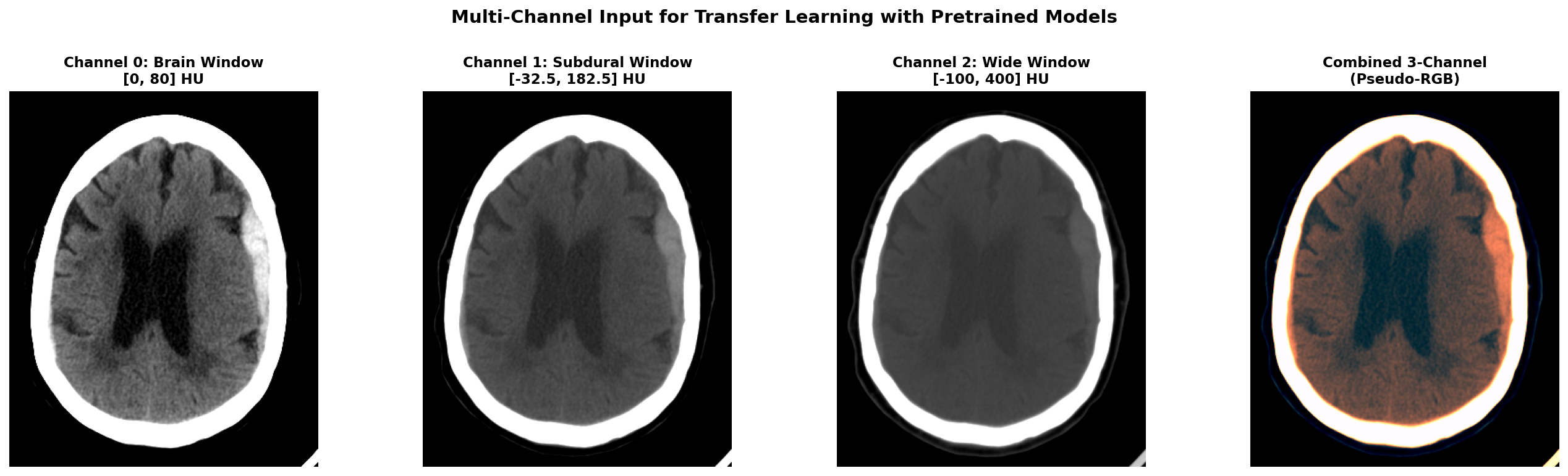
To leverage ResNeXt's RGB pretrained weights on our grayscale CT data, I created a 3-channel input using different CT window settings, each emphasizing different tissue types and pathological features. The first channel used a brain window with center 40 HU and width 80 HU, optimized for viewing gray and white matter parenchyma. The second channel employed a subdural window with center 75 HU and width 215 HU, specifically enhanced for detecting blood and hemorrhage. The third channel used a wide window spanning -100 to 400 HU to provide broad tissue context including bones and soft tissues.
For each window, we define a center value and width, then calculate the minimum value as center minus half width and maximum value as center plus half width. We clip the image HU values to this range and normalize to the 0-1 interval. By stacking these three differently-windowed versions of the same slice, we create a pseudo-RGB input that mimics the structure of natural images while preserving clinically relevant information at different intensity scales.
Training Strategy
The model was trained using weighted cross-entropy loss to handle the significant class imbalance in the dataset, where control cases and certain hemorrhage subtypes were dramatically more common than others. Data augmentation included horizontal flips, which are appropriate given the approximate symmetry of the brain, small rotations to account for patient positioning variations, and brightness and contrast adjustments to simulate different scanner calibrations and improve model robustness.
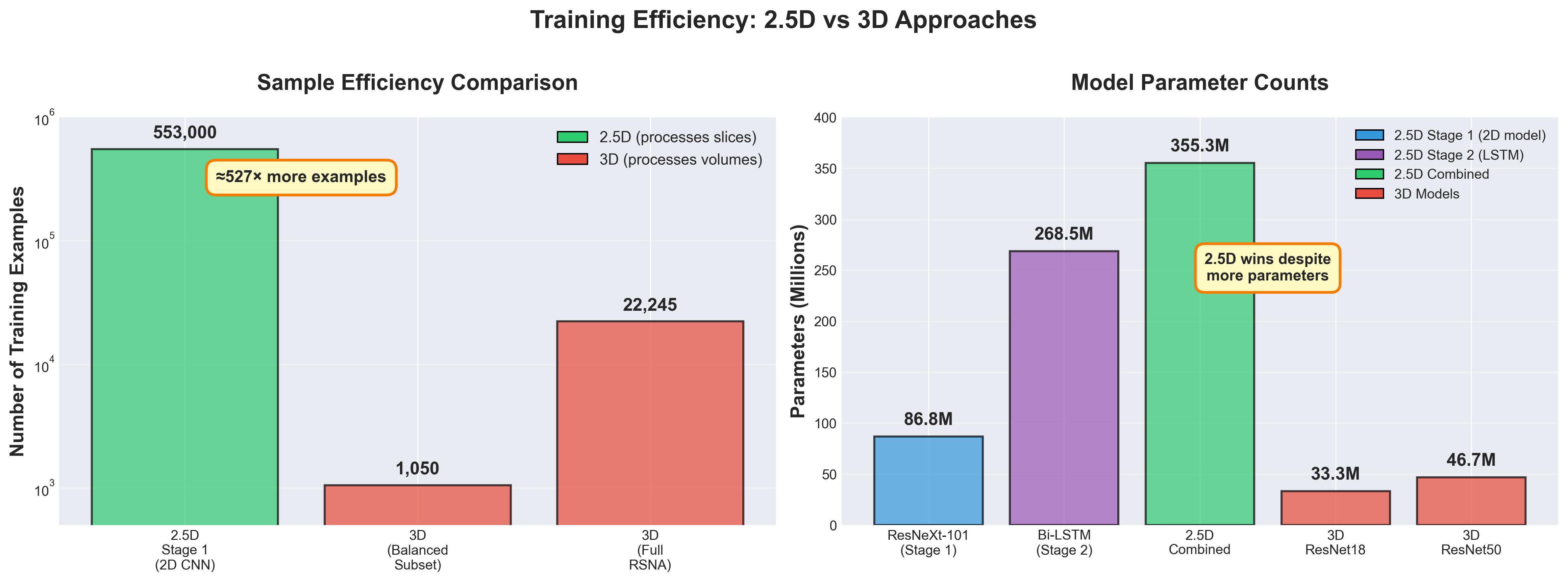
Critically, the full RSNA training set of approximately 553,000 slices was used for Stage 1 training. This represents a massive increase in effective sample size compared to the 1,050 volumes used for 3D training—each slice becomes an independent training example rather than each entire volume. This dramatic improvement in sample efficiency would prove crucial to the model's success.
Stage 1 Results
When I evaluated the model using direct predictions with a threshold of 0.5 on the sigmoid outputs, the results were initially disappointing with a slice-wise F1 of only 0.460. This was barely better than the failed 3D models and left me concerned that even this new approach might not work.
However, I decided to try a different evaluation strategy using the learned embeddings rather than the classification predictions. For each test slice, I extracted the 2048-dimensional embedding from the penultimate layer and computed cosine similarity to the mean embeddings of each class in the training set. The slice was assigned to the class with highest cosine similarity. This embedding-based approach achieved dramatically different results: slice-wise F1 of 0.837 and volume-wise F1 of 0.893 when aggregating slice predictions using max pooling.
The poor performance with direct thresholding suggested that while the model was learning discriminative features, the predicted probabilities weren't well-calibrated for binary decisions at the 0.5 threshold—a common issue with transfer learning where the final classification layer is randomly initialized. However, the learned embeddings were highly discriminative, capturing subtle features that reliably separated different stroke types. This insight proved crucial—the penultimate layer representations contained far more useful information than the raw classification predictions, suggesting that the feature extractor was working excellently even though the classifier head needed improvement.
Stage 2: Bi-directional LSTM Sequence Model
Architecture and Rationale
Stage 2 treats each CT volume as a temporal sequence of slices, directly analogous to how natural language processing treats sentences as sequences of words or how video analysis treats clips as sequences of frames. The input consists of the sequence of 2048-dimensional embedding vectors from Stage 1, one for each slice in the volume ordered from cranial to caudal. Delta features - being the difference between two consecutive slices - are concatenated to the embeddings, tripling the input dimension to 6144 and helping the model detect inter-slice changes.
The core of the model is a 2-layer bidirectional LSTM with 2048 hidden units per direction, compressing the 6144-dimensional input into a more compact representation that acts as regularization. The forward LSTM processes slices from top to bottom of the brain, while the backward LSTM processes them in the opposite direction from bottom to top. This bidirectional processing is crucial because stroke lesions can have contextual clues both above and below them in the scan. For example, a faint abnormality on one slice might be confirmed by clearer pathology on adjacent slices in either direction.
The bidirectional architecture allows each slice's prediction to be informed by the full volumetric context rather than just preceding slices in one direction. This mimics the radiologist workflow of scrolling back and forth through the volume to confirm initial impressions, looking for supporting evidence in both directions from a suspicious finding. The model produces both slice-wise predictions for each individual slice and an aggregated volume-level prediction obtained through max pooling, operating under the reasonable assumption that if any slice in a volume shows strong evidence of a particular stroke type, the entire volume should be classified accordingly.
Training Strategy
The Stage 2 model was trained on fixed embeddings extracted from the pretrained Stage 1 model. Importantly, the Stage 1 weights were frozen and not fine-tuned during Stage 2 training. This two-stage approach dramatically simplified optimization by decoupling the feature learning (Stage 1) from the sequence modeling (Stage 2), allowing each stage to be tuned independently without competing gradients.
The loss function was cross-entropy computed on slice-level predictions, providing dense supervision at every position in the sequence rather than only at the volume level. For volume-level classification, max pooling was applied over all slice predictions, based on the clinical intuition that even a single slice showing clear hemorrhage should classify the entire scan as hemorrhagic.
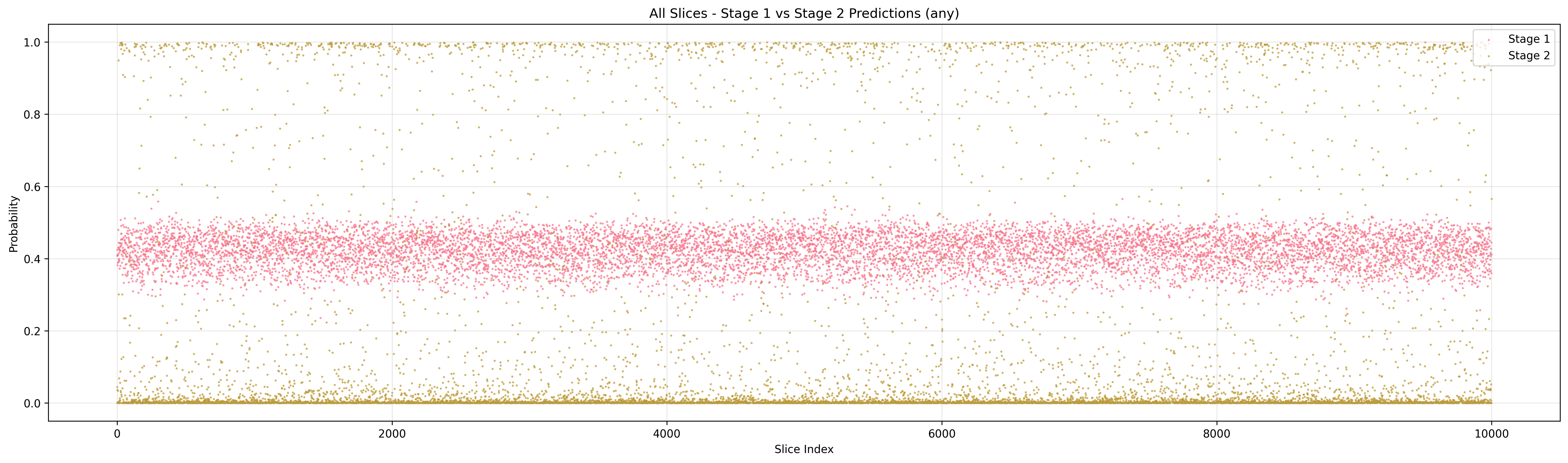
Stage 2 Results: The Breakthrough Moment
The LSTM Stage 2 model achieved slice-wise F1 of 0.857 and volume-wise F1 of 0.945 on the validation set. Compared to Stage 1's embedding-based results of slice F1 0.837 and volume F1 0.893, this represented a meaningful 2.0% improvement in slice predictions and a substantial 5.2% improvement in volume-level classification.
This was the moment when everything clicked into place. Detailed analysis of the predictions revealed that the LSTM was correcting many false negatives from Stage 1 by learning that hemorrhages typically span multiple consecutive slices. If Stage 1 missed a hemorrhage on one slice but detected it on two adjacent slices, the LSTM could use this sequential pattern to correct the isolated error. The volume-level F1 of 0.945 was excellent by medical imaging standards—dramatically better than any 3D model I'd trained, and achieved with an architecture that was faster and more stable to train.
Could Transformers Do Even Better?
Motivation
The LSTM results were excellent and validated the 2.5D staged approach, but I wondered whether more sophisticated sequence models might push performance even higher. Transformers have revolutionized natural language processing through their attention mechanisms that can model long-range dependencies more effectively than LSTMs' gated recurrent connections. Could a transformer-based Stage 2 model outperform the LSTM by learning more complex patterns across the slice sequence?
Transformer Variants Tested
I experimented with four different transformer architectures, each designed to test different hypotheses about what makes sequence modeling effective for medical volumes. The Standard Transformer used a vanilla encoder architecture with sinusoidal positional encoding to inject information about absolute slice position in the volume. The Hierarchical Transformer processed slices in groups of consecutive slices, allowing it to capture both local patterns within small neighborhoods and global patterns across the entire volume through hierarchical aggregation.
The Enhanced Transformer incorporated multi-scale attention with separate attention heads dedicated to local context (adjacent slices) and global context (entire volume), plus learnable positional encodings that could adapt to the specific spatial statistics of CT volumes. Finally, I tested Mamba2, a recent state space model with linear complexity that promises better efficiency for long sequences while maintaining strong modeling power through its selective state spaces.
Results and Insights
The results showed modest improvements but no dramatic gains over the simpler LSTM. The Standard Transformer achieved slice F1 of 0.862 and volume F1 of 0.945, matching the LSTM's volume performance while slightly improving slice-level predictions by 0.5%. The Hierarchical Transformer actually performed slightly worse with slice F1 of 0.852 and volume F1 of 0.934, suggesting that grouping slices may have lost some important fine-grained spatial information.
The Enhanced Transformer with multi-scale attention achieved the highest volume F1 of 0.947, marginally better than LSTM, with slice F1 of 0.860. The Mamba2 model achieved slice F1 of 0.854 and volume F1 of 0.941, competitive but not superior to the baseline LSTM.
| Architecture | Slice F1 | Volume F1 |
|---|---|---|
| Bi-LSTM (baseline) | 0.857 | 0.945 |
| Standard Transformer | 0.862 | 0.945 |
| Hierarchical Transformer | 0.852 | 0.934 |
| Enhanced Transformer | 0.860 | 0.947 |
| Mamba2 | 0.854 | 0.941 |
The Enhanced Transformer's volume F1 of 0.947 represented the highest performance achieved, but the gain over the simpler LSTM (0.945) was minimal—just 0.2 percentage points. The LSTM remained highly competitive with a simpler architecture, faster training time due to operating on fixed embeddings (no backpropagation through Stage 1), and fewer hyperparameters requiring tuning.
The critical insight from these experiments is that the 2.5D staged approach itself was the key innovation that enabled strong performance. The choice of sequence model for Stage 2, whether LSTM, Transformer, or more exotic architectures, mattered far less than the overall paradigm shift from attempting to train 3D models from scratch to leveraging powerful 2D pretrained models combined with sequence modeling over learned embeddings. For further improvements, it seems the stage 1 feature extractor is the most promising area to explore, as it provides the foundational representations upon which all subsequent modeling depends and is the primary bottleneck limiting overall performance.
Why Does 2.5D Win? Understanding the Trade-offs
The experimental results clearly demonstrate that 2.5D consistently outperformed 3D approaches. But understanding why requires diving into the fundamental trade-offs between these architectural choices.
1. The Curse of Dimensionality
Data Requirements Scale With Dimension
More parameters fundamentally require more training samples to avoid overfitting and learn generalizable features. But the curse of dimensionality goes deeper than just parameter counts—it creates exponential data sparsity that makes comprehensive feature space coverage practically impossible.
Consider a simple thought experiment about sampling density. To adequately cover a 1D feature space, you might need samples covering 20% of the range. But for 2D, you'd need 45% coverage per dimension (since 0.45² ≈ 0.20) to maintain the same density. For 3D, this jumps to 58% per dimension (0.58³ ≈ 0.20). As dimensions increase, the required training data grows exponentially to maintain adequate coverage of the feature space. This isn't just a theoretical concern—it has profound practical implications for 3D medical imaging.
For medical CT volumes, this problem becomes severe. A preprocessed 3D volume of 64×128×128 voxels exists in an astronomically large feature space. Even with 22,245 training volumes, the data points become vanishingly sparse, like trying to understand the ocean by examining a few droplets of water. The model must interpolate across vast empty regions of feature space where it has never seen training examples, making generalization extraordinarily difficult.
The 2.5D approach sidesteps this trap through dimensionality reduction. Stage 1 operates on individual 2D slices with 256×256 = 65,536 dimensions rather than full 3D volumes with 64×128×128 = 1,048,576 dimensions—a 16× reduction in input dimensionality. More critically, with 553,000 training slices versus 22,245 training volumes, the ratio of training samples to feature dimensions is dramatically different: approximately 8.4 samples per dimension for 2D versus only 0.02 samples per dimension for 3D. To achieve the same feature space coverage density as the 2D approach, 3D training would require approximately 8.8 million volumes—nearly 400× more data than available in the RSNA dataset.
Computational Cost and Memory
3D operations are computationally expensive in practice. Memory consumption grows dramatically because 3D feature maps occupy much more GPU memory than 2D feature maps, severely limiting batch sizes. A 2D feature map of size 128×128 with 64 channels requires 128 × 128 × 64 = 1,048,576 values. The 3D equivalent with 64 slices requires 64 × 128 × 128 × 64 = 67,108,864 values—64 times more memory.
This memory bottleneck forces smaller batch sizes for 3D models, which hurts training stability and makes it harder to use batch normalization effectively. Training time per epoch increases by 5-10× for 3D models compared to 2D, not just because of more parameters but because of the computational complexity of 3D convolutions and the inability to batch examples efficiently.
2. Transfer Learning is a Superpower
The 2.5D approach leverages massive-scale 2D pretrained models in a way that 3D models simply cannot match currently. ResNeXt-101 was pretrained on 940 million weakly-supervised Instagram images. Standard ResNets use ImageNet pretraining on 1.2 million carefully annotated natural images. These models have learned incredibly robust low-level features like edge detectors, texture recognizers, and shape detectors that transfer remarkably well to medical imaging, despite the dramatic domain shift from natural images to CT scans.
The transfer learning effect is profound. The pretrained model starts with feature detectors that already work reasonably well for detecting edges, textures, and basic shapes in medical images. Fine-tuning adapts these features to the medical domain, requiring far less data than learning from scratch. The embedding quality achieved by Stage 1 (F1 0.837 on slices) using pretrained weights vastly exceeded what any randomly initialized model achieved.
In stark contrast, 3D pretrained models are rare and limited in scope. MedicalNet, the most comprehensive effort I found, was trained on only 23 medical datasets—orders of magnitude less data than ImageNet or weakly-supervised Instagram. My experiments confirmed that MedicalNet pretraining (F1 0.813) substantially improved over random initialization (F1 0.418) but still fell far short of 2D pretraining (F1 0.945).
The asymmetry in available pretraining is a structural advantage for 2.5D that's unlikely to change soon. Natural images are abundant and easy to collect at massive scale. Medical 3D volumes are scarce, expensive to acquire, and require expert annotation. Until massive 3D medical pretraining datasets exist, 2.5D will maintain this fundamental advantage.
3. Inductive Biases: Slices vs Volumes
Radiologist Workflow Alignment
Radiologists read CT scans slice-by-slice, scrolling through the volume while building a mental 3D model. They identify suspicious regions on individual slices, then look at adjacent slices for confirmation and to understand the 3D structure. The 2.5D staged approach directly mimics this proven workflow: Stage 1 identifies suspicious features on individual slices (like a radiologist's first pass), and Stage 2 integrates context from neighboring slices (like scrolling for confirmation).
This alignment with expert practice isn't just philosophically satisfying—it's a good inductive bias. The human visual system and expert training have evolved to process medical images this way because it works well given the structure of the data and task. Building models that follow similar processing patterns can be advantageous.
Anisotropic Resolution
CT scans have fundamentally different resolution in different dimensions. In-plane resolution (x-y dimensions within a slice) is typically 0.5-1 mm, providing fine detail for visualizing small structures. Slice spacing (z dimension between slices) is typically 2-5 mm, much coarser than the in-plane resolution. This anisotropy means that the z-axis is fundamentally different from x and y.
3D convolutions with 3×3×3 kernels treat all three dimensions equally, averaging features across x, y, and z with equal weights. This may not be appropriate given the anisotropic resolution—averaging features across 3 pixels in x or y (spanning 1.5-3 mm) is very different from averaging across 3 slices in z (spanning 6-15 mm). The 2.5D approach naturally handles this anisotropy by processing x-y dimensions with 2D convolutions and modeling the z dimension separately with sequence models designed for more coarse-grained dependencies.
4. Sample Efficiency: The Hidden Advantage
The sample efficiency difference between 2.5D and 3D is perhaps the most underappreciated factor in explaining the performance gap. With 2.5D, each individual slice becomes a training sample for Stage 1. A volume containing 100 slices provides 100 training examples for learning slice-level features. With 3D, each complete volume is a single training sample. That same patient provides only 1 example for learning volumetric features.
This represents an approximately 500× increase in effective sample count for Stage 1 training. With 1,050 volumes in the balanced subset, 3D training has 1,050 samples. With those same volumes containing an average of 70 slices each, 2.5D Stage 1 training has approximately 73,500 samples. With the full RSNA training set of 22,245 volumes, 2.5D has access to approximately 553,000 slice-level training samples.
This massive increase in sample count allows Stage 1 to learn robust slice-level features that generalize well. The success of Stage 1 embeddings (F1 0.837) compared to 3D models (F1 0.418) can be largely attributed to this sample efficiency advantage combined with transfer learning.
Stage 2 then operates at the volume level on only 1,050 or 22,245 volumes, but it's learning a much simpler task: how to aggregate already-good slice-level features into volume-level predictions. This is far easier than learning discriminative volumetric features from scratch, requiring far less data.
Conclusion
This experimental journey challenged a core assumption: that 3D models are inherently superior for volumetric medical data. The final results tell a different story. A 2.5D staged approach combining ResNeXt-101 with bidirectional LSTM achieved F1=0.945 on volume-level stroke classification, while 3D models trained from scratch plateaued at F1=0.418 despite extensive architecture search and hyperparameter tuning across ResNet and DenseNet variants.
The performance gap stems from fundamental factors rather than implementation details. First, sample efficiency creates a 527× advantage for 2.5D: the full RSNA training set provides 553,000 independent slice-level examples for Stage 1 compared to only 1,050-22,245 volume-level examples for 3D models. Second, transfer learning from 940 million weakly-supervised Instagram images provides ResNeXt-101 with robust pretrained features that transfer remarkably well to medical imaging despite the domain shift. Third, the 2.5D approach has 355M parameters compared to 33M for 3D ResNet18, yet trains more stably by decoupling feature learning (Stage 1) from sequence modeling (Stage 2), allowing independent optimization of each stage without competing gradients.
The literature's emphasis on 3D superiority often relies on private datasets, massive data scales, or segmentation tasks where 3D spatial consistency is critical. My results demonstrate that for classification with limited data—even 22,245 volumes, considered large by medical imaging standards—architectural choices must account for available pretraining, sample efficiency, and optimization complexity. The "best" architecture depends critically on task requirements and resource constraints, not theoretical arguments alone.
For practitioners facing similar decisions, empirical validation on your specific dataset outweighs literature intuitions. Pure 2D slice-wise approaches work when inter-slice dependencies are weak and slice-level labels are abundant. The 2.5D staged approach excels for classification tasks with moderate data (1,000-100,000 volumes), leveraging massive 2D pretraining while capturing volumetric context through sequence models. Native 3D convolutions remain essential for dense segmentation where reconstructing 3D masks from 2D predictions creates boundary artifacts, or when datasets exceed 100,000 volumes with sufficient positive examples to overcome the curse of dimensionality.
Several technical insights emerged from failed experiments. When 3D models underperformed, sanity checks on toy datasets (cat vs dog classification) isolated the problem to medical data characteristics rather than implementation bugs. Stage 1's learned embeddings with cosine similarity (F1=0.837) vastly outperformed direct classification predictions (F1=0.460), revealing that transfer learning's randomly initialized classification head was poorly calibrated despite the feature extractor learning discriminative representations. External validation on CQ500 exposed models learning scanner-specific artifacts rather than medical features, demonstrating the critical need for cross-dataset testing before clinical deployment.
Starting with minimal viable models proved essential for systematic debugging. The dual-task 3D U-Net combining classification and segmentation introduced too many confounding factors simultaneously, making failure diagnosis impossible. Simplifying to pure classification isolated the fundamental challenge: 3D models require far more data than available to learn from scratch, regardless of architectural complexity. This lesson applies broadly—add complexity only with empirical justification, never as a starting point.
The dimension dilemma taught me that theory guides but experiments decide. I began this work convinced 3D was correct based on solid reasoning and literature support, yet the data showed otherwise through dozens of failed experiments. For anyone working on medical imaging problems, question your assumptions, benchmark multiple approaches empirically, and document failures alongside successes. Deep learning in healthcare carries real consequences for patient lives. We advance faster by sharing both instructive failures and polished successes, helping the community avoid dead ends while building on what works.
References
-
J. Fan et al., "Dual-task vision transformer for rapid and accurate intracerebral hemorrhage CT image classification", Scientific Reports, vol. 14, no. 1, Nov. 2024, doi: 10.1038/s41598-024-79090-y
-
S. Kyung et al., "Improved performance and robustness of multi-task representation learning with consistency loss between pretexts for intracranial hemorrhage identification in head CT", Medical Image Analysis, vol. 81, p. 102489, Oct. 2022, doi: 10.1016/j.media.2022.102489.
-
Y. Zhou et al., "Multi-task learning for segmentation and classification of tumors in 3D automated breast ultrasound images", Medical Image Analysis, vol. 70, p. 101918, May 2021, doi: 10.1016/j.media.2020.101918.
-
Kaggle RSNA 2019 Competition. (2019). 2nd Place Solution: Sequential Model for Intracranial Hemorrhage Detection. https://www.kaggle.com/competitions/rsna-intracranial-hemorrhage-detection/writeups/nobrainer-2nd-place-solution-sequential-model
-
A. E. Flanders et al., "Construction of a Machine Learning Dataset through Collaboration: The RSNA 2019 Brain CT Hemorrhage Challenge", Radiology: Artificial Intelligence, vol. 2, no. 3, p. e190211, May 2020, doi: 10.1148/ryai.2020190211.
-
Liang, G., & Zheng, L. (2019). AISD: Ischemic stroke lesion segmentation dataset. GitHub repository. https://github.com/GriffinLiang/AISD
-
D. Umerenkov, S. Kudin, M. Pekshevaand D. Pavlov, "CPAISD: Core-Penumbra Acute Ischemic Stroke Dataset". Zenodo, Mar. 28, 2024. doi: 10.5281/zenodo.10892316
-
M. Ayoub, et al. "End to end vision transformer architecture for brain stroke assessment based on multi-slice classification and localization using computed tomography", Computerized Medical Imaging and Graphics, vol. 109, p. 102294, Oct. 2023, doi: 10.1016/j.compmedimag.2023.102294.
-
A. Neethi, et al., "Stroke classification from computed tomography scans using 3D convolutional neural network", Biomedical Signal Processing and Control, vol. 76, p. 103720, July 2022, doi: 10.1016/j.bspc.2022.103720.
-
A. Gautam and B. Raman, "Towards effective classification of brain hemorrhagic and ischemic stroke using CNN", Biomedical Signal Processing and Control, vol. 63, p. 102178, Jan. 2021, doi: 10.1016/j.bspc.2020.102178.
Acknowledgments
This research used three publicly available datasets. The RSNA 2019 Brain CT Hemorrhage Challenge dataset is available on Kaggle. The AISD dataset can be accessed on GitHub. The CPAISD dataset is hosted on Zenodo. Special thanks to the organizers of the RSNA 2019 Kaggle competition whose solution architectures inspired the 2.5D staged approach. The multi-task 3D modeling approach drew on insights from recent papers on dual-task learning in medical imaging. Special thanks to JD Wuarin and Kevish Napal for their valuable feedback and support throughout this project.
For questions or discussions, feel free to reach out through the comments or connect with me directly.