Understanding and Processing CT Imaging for Stroke Detection

This post aims to guide you through the steps of processing medical images. Drawing from research experience with stroke detection, the methods presented here will focus on stroke detection from CT scans but can be the starting point for analyzing other organ CT images or other imaging modalities (e.g CTA,CTP, MRI).

A) The starting point of any reliable medical imaging application: quality datasets

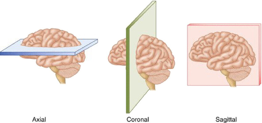
Computed tomography (CT), or more precisely non-contrast CT (NCCT), is the most common imaging modality used in emergency settings to diagnose strokes due to its speed and effectiveness. Images are acquired by rotating an X-ray tube around the patient while sampling transmitted photons with a ring of detectors without injecting any contrast agent. Then, the images are reconstructed using algorithms to create cross-sectional views of the brain. The most common view is the axial plane, which is a horizontal slice parallel to the ground. Other views like coronal (vertical plane separating front and back) and sagittal (vertical plane separating left and right) can be reformatted from the axial slices. An image speaks a thousand words, so here is an example of axial CT slices from a stroke patient showing both ischemic and hemorrhagic lesions in Figure 1.

Now, what is a stroke and why study it? Cerebrovascular accident, most commonly known as **stroke**, occurs when blood flow to a part of the brain is interrupted or reduced, preventing brain tissue from receiving the oxygen and nutrients it needs. It is the second leading cause of death globally among non-communicable disorders. 1 in 4 adults over 25 years old will have a stroke in their lifetime. This apparently common health issue is one of the deadliest, highlighting the critical importance of understanding and improving current treatment of this condition. There are 2 main types of strokes: **ischemic** and **hemorrhagic**. Ischemic strokes are caused by a blockage in a blood vessel, preventing blood flow to the brain, while hemorrhagic strokes result from a ruptured blood vessel causing bleeding in or around the brain. The treatment for these two types of strokes is fundamentally different, making accurate and rapid diagnosis crucial. CT scans are the primary imaging modality used in emergency settings to differentiate between these stroke types due to their speed and effectiveness in detecting hemorrhages.

Datasets for CT images are quite rare and of small size because they often require doctors to label a vast quantity of images by hand, thus taking a long time and being expensive. This represents a great challenge as most deep learning techniques require a great amount of data to reach good performance if trained from scratch. If you add to that the fact that most papers published on the subject use private datasets of small sizes (~ 500 scans), this can be quite challenging to get your hands on the right amount and quality of data to train machine learning models. Luckily, some open datasets of quality exist. I listed trusted datasets for stroke detection applications I noticed in Table 1.

Table 1. Overview of publicly available stroke imaging datasets referenced in this work.

Dataset	Size	Stroke Type	Key Features	License	Link
RSNA 2019	25,000+ scans 700,000+ slices	Hemorrhagic + Control	NCCT 5 hemorrhage subtypes 60+ radiologist annotations	Non-commercial use only	Kaggle Paper
CPAISD	112 scans	Ischemic (acute)	NCCT Penumbra & core delineation Within 24h of symptoms	Research use	Zenodo Paper
AISD	397 scans	Ischemic (acute)	Paired NCCT-MRI (DWI) Manual lesion contours Within 24h of symptoms	Non-commercial use only	GitHub
CQ500	491 scans 193,317 slices	NCCT Hemorrhagic + Other pathologies + Control	5 hemorrhage subtypes 3 radiologist reads	CC BY-NC-SA 4.0	Dataset Paper
CODEC-IV	159 scans	Ischemic	CTA Large vessel occlusion	Request-based access	Paper GitHub
APIS	96 scans	Ischemic	Paired NCCT + ADC 2 expert radiologist annotations	CC BY 4.0	Challenge Paper
UniToBrain	258 scans	Ischemic	CT perfusion maps Core vs penumbra	CC BY 4.0	IEEE DataPort Paper

When choosing a dataset, consider your specific task requirements. RSNA 2019 is an evident choice for hemorrhage detection with its massive size, but suffers from class imbalance. For ischemic stroke detection, AISD offers the advantage of paired MRI ground truth, addressing the challenge that NCCT has low detection-rate in early ischemia, making the labeling of the data with MRI more accurate. CPAISD is particularly valuable for the most challenging scenario: hyperacute stroke where NCCT shows minimal signs. For comprehensive diagnosis, CQ500 provides some images also presenting brain pathologies like a cranial fracture. Note that CODEC-IV and UniToBrain use different imaging modalities (CTA and CTP respectively) requiring distinct processing pipelines from standard NCCT. Finally, smaller datasets like APIS (96 scans) are insufficient for training from scratch but valuable for transfer learning validation or can serve as external test sets.

B) DICOM: a standardized image format for medical imaging

DICOM stands for Digital Imaging and Communications in Medicine, a comprehensive international standard that revolutionized how medical images are stored, transmitted, and processed across healthcare systems. Developed in the 1980s by the American College of Radiology (ACR) and the National Electrical Manufacturers Association (NEMA), DICOM emerged from the necessity to standardize communication between different medical imaging equipment manufacturers. Before DICOM, each vendor had proprietary formats, making it nearly impossible for hospitals to integrate imaging systems from different companies. Moreover, CT scanners, MRI machines, and other modalities generate not just pixel data, but also important contextual information about patient positioning, acquisition parameters, and technical specifications. DICOM combines both the image data and all associated metadata into a single file, ensuring that contextual information is not lost during transfer or storage.

DICOM File Architecture: Metadata and Pixel Data Integration

A DICOM file consists of two primary components: an extensive metadata header and the actual pixel data. The metadata header contains a structured collection of data elements, each identified by unique tags in the format (Group, Element), such as (0010,0010) for patient name or (0028,0030) for pixel spacing. This header stores patient demographics, study information, acquisition parameters, image dimensions, and technical specifications required for proper image display and interpretation.

The pixel data follows the metadata, stored in a special attribute (7FE0,0010) that contains the actual image information as raw bytes. Unlike standard image formats that prioritize file size, DICOM preserves the original bit depth and dynamic range captured by the imaging equipment, ensuring no diagnostic information is lost through compression artifacts. This pixel data can be uncompressed or utilize medical-grade compression standards like lossless JPEG or JPEG 2000.

Essential DICOM Fields for Data Processing

A DICOM file contains a large number of metadata fields, but only a subset is essential for processing medical images for stroke detection. We can organize these fields by their purpose and complexity level.

At the highest level, we need unique identifiers to track patients and scans while avoiding data leakage during model training. One important concept: CT scanners acquire slices (individual 2D images taken at different positions along an axis) which may later be reconstructed into a 3D volume. Therefore, we have different levels of identification:

It is possible to uniquely identify a single patient across all their medical imaging studies using PatientID
It is possible to uniquely identify a single slice (a 2D image corresponding to a specific cross-section through the body) using SOPInstanceUID
It is possible to uniquely identify a scan (the complete group of slices acquired together with the same settings and protocol) using SeriesInstanceUID
It is possible to uniquely identify a study (which may contain multiple scans, reconstructed images along different axes, or scans with different slice thicknesses) using StudyInstanceUID

The relationship forms a hierarchy: one StudyInstanceUID can contain multiple SeriesInstanceUID, and each SeriesInstanceUID typically contains multiple SOPInstanceUID representing individual slices.

At an intermediate level, there are fields that describe basic image properties that help verify dataset consistency. The Modality field tells us what type of imaging was performed (CT, MRI, etc.), while Rows and Columns specify the image dimensions in pixels. The PhotometricInterpretation field defines how pixel values should be interpreted for visualization - for CT scans this is typically MONOCHROME2 (higher pixel values = brighter) or MONOCHROME1 (the inverse). These fields ensure we're working with the correct type of data and that our dataset is homogeneous.

At an even lower level, there are fields describing how the image was acquired in physical space. PixelSpacing defines the physical distance between pixel centers in millimeters, which can vary between slices in a single series. ImagePositionPatient provides the x, y, z coordinates of the upper-left corner of each slice in the patient's coordinate system - essential for correctly ordering slices along the z-axis when reconstructing 3D volumes. ImageOrientationPatient describes the orientation of the slice relative to the patient's body, useful for accurate spatial representation.

Finally, for CT images, the pixel values need to be converted to Hounsfield Units (HU) for meaningful interpretation. Hounsfield Units are a standardized scale used in CT imaging to represent tissue density relative to water. By definition, water = 0 HU and air = –1000 HU, with other tissues (bone, fat, etc.) assigned values based on their X-ray attenuation.

Table 2 below summarizes all these essential DICOM fields with their technical identifiers:

Table 2. Essential DICOM metadata fields for CT image processing and stroke detection.

Field Name	DICOM Tag	Purpose Category	Description
PatientID	(0010,0020)	Unique Identifiers	Identifies the patient across all imaging studies
SOPInstanceUID	(0008,0018)	Unique Identifiers	Uniquely identifies a single 2D slice (SOP = Service-Object Pair)
SeriesInstanceUID	(0020,000E)	Unique Identifiers	Uniquely identifies one complete scan (all slices acquired with same settings)
StudyInstanceUID	(0020,000D)	Unique Identifiers	Uniquely identifies a medical imaging study (may contain multiple scans)
Modality	(0008,0060)	Basic Image Properties	Type of imaging (CT, MR, etc.)
Rows	(0028,0010)	Basic Image Properties	Image height in pixels
Columns	(0028,0011)	Basic Image Properties	Image width in pixels
PhotometricInterpretation	(0028,0004)	Basic Image Properties	Defines pixel value mapping (MONOCHROME2: higher values = brighter; MONOCHROME1: inverse; RGB or YBR_FULL for color)
PixelSpacing	(0028,0030)	Spatial Information	Physical distance between pixel centers in millimeters [row spacing, column spacing]
ImagePositionPatient	(0020,0032)	Spatial Information	X, Y, Z coordinates of the upper-left pixel in patient coordinate system (mm)
ImageOrientationPatient	(0020,0037)	Spatial Information	Direction cosines defining slice orientation relative to patient anatomy
RescaleIntercept	(0028,1052)	HU Conversion (CT-specific)	Intercept parameter for converting raw pixel values to Hounsfield Units
RescaleSlope	(0028,1053)	HU Conversion (CT-specific)	Slope parameter for converting raw pixel values to Hounsfield Units

Working with PyDicom: Practical Implementation

The PyDicom library provides an intuitive Python interface for DICOM manipulation, making it the de facto standard for medical imaging research. Reading a DICOM file is straightforward:

import pydicom
import matplotlib.pyplot as plt

ds = pydicom.dcmread('path/to/ct_scan.dcm') # load DICOM file

# How to access metadata
print(f"Modality: {ds.Modality}")
print(f"Image Dimensions: {ds.Rows} x {ds.Columns}")

# Extract pixel data
pixel_array = ds.pixel_array

# Display the image
plt.imshow(pixel_array, cmap='gray')
plt.title(f"CT Slice")
plt.show()

C) Step-by-Step Processing of CT Images for Stroke Detection

For the following examples, we'll use a real CT scan from the RSNA 2019 Brain CT Hemorrhage Challenge Dataset, specifically showing a case of hemorrhagic stroke. This allows us to demonstrate each processing step on actual clinical data where blood is visible in the brain tissue due to a ruptured vessel.

Processing CT images for stroke detection involves several common steps to ensure that the data is in the optimal format for training deep learning models. Keep in mind that these steps can be adapted based on the specific requirements of your project, dataset or task and no real standard exists.

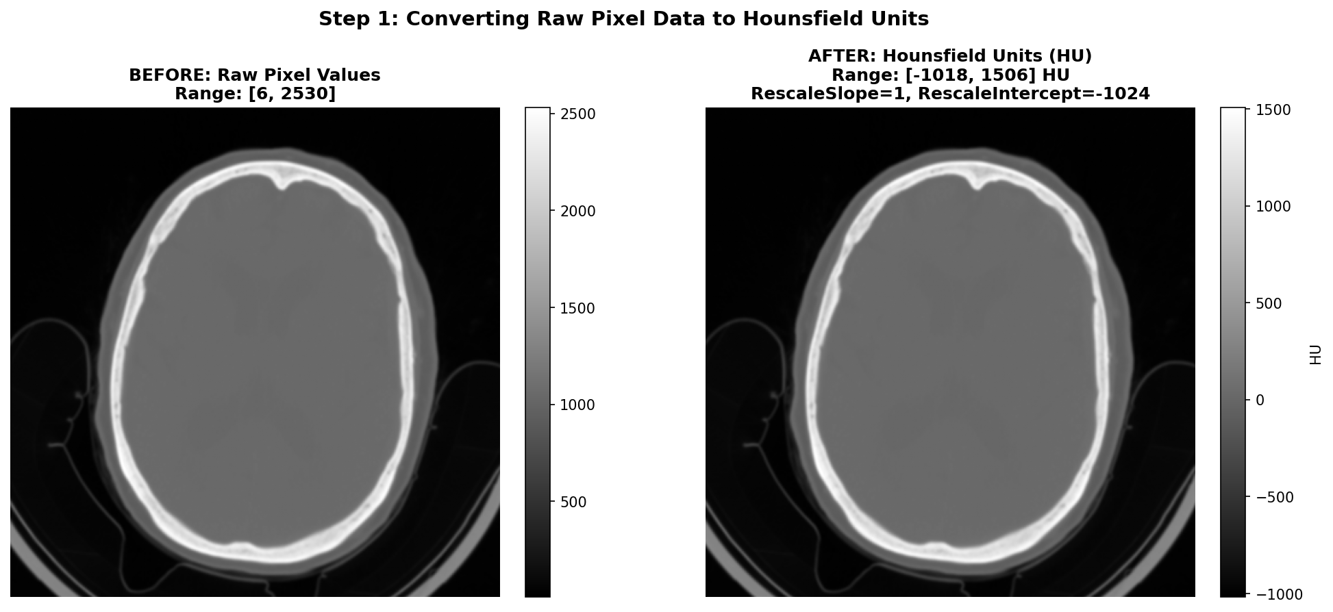
1) Converting the raw data to Hounsfield Units (HU)

As said before, CT images are stored in DICOM files with pixel values that need to be converted to Hounsfield Units (HU) for meaningful interpretation. This conversion is essential because HU provides a standardized scale for tissue density, which is crucial for identifying abnormalities such as hemorrhages or ischemic regions in the brain. To give you a better idea of the HU scale, the air is -1000 HU, water is 0 HU, and bones can range from +200 to more than 1000 HU. Useful tissues like blood vessel tissues or grey matter are generally between -50 and +200 HU. The conversion is done using the Rescale Slope and Rescale Intercept values found in the DICOM metadata. The transformation is applied using an affine equation:

$HU = (Pixel Value * Rescale Slope) + Rescale Intercept$

Common values for Rescale Slope and Intercept are 1 and -1024 respectively - in order to shift the air pixel value from 0 to around -1000 HU, though it is important to check these values for each DICOM file as they can vary between different scanners or acquisition protocols.

The figure below shows the conversion process on our hemorrhagic stroke series example from the RSNA dataset. On the left, we see the raw pixel values as stored in the DICOM file - which are not intended for direct visualization. On the right, after applying the HU conversion formula with RescaleSlope=1 and RescaleIntercept=-1024, the values are properly scaled to the Hounsfield scale and we can see the image properly.

2) Reconstructing the brain volume from 2D slices

This step is optional and only required if you want to work with 3D data. It is not required if you want to work with 2D slices only, though you will lose the spatial context between slices and thus some information. It is also often useful to reconstruct volume data in order to either visualize it or make predictions on the whole volume and not only slice by slice which makes more sense in a real clinical setting. Indeed, the end goal is to be able to diagnose a patient well, having at your disposal the whole scan containing all the slices taken during the exam acquisition.

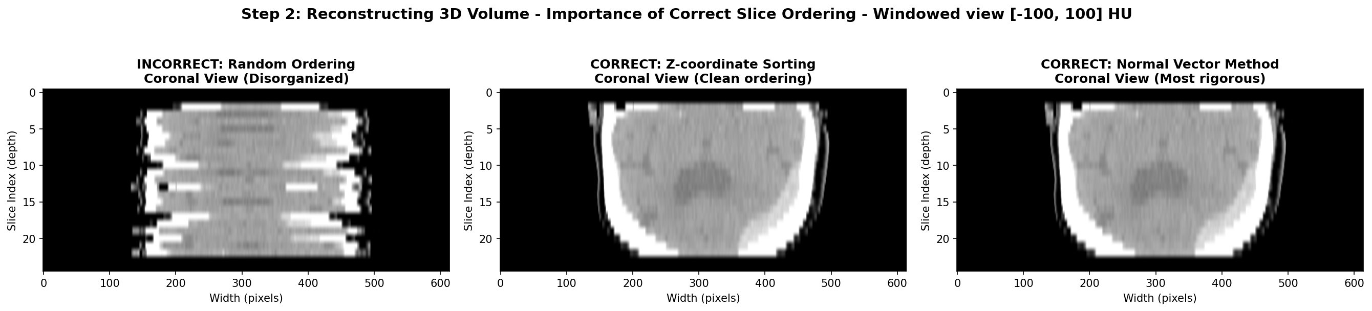
In order to achieve a proper reconstruction, one first needs to group the slices that belong to the same scan. In some datasets they are already contained in the same folder but it is always safer to group them using DICOM metadata. This can be done using the SeriesInstanceUID DICOM field. Since a series designate a set of slice from the same acquisition, it is a foolproof method to group your slices that way.

Then, the slices need to be ordered and stack along the axis perpendicular to the slice plane, usually the z-axis due to the commonly used axial acquisition plane - plane parallel to the ground. One must be careful to not use unreliable DICOM fields like SliceLocation or InstanceNumber. In my experience, they can be wrong and often missing for some slices. Instead, the most reliable method is to use the ImagePositionPatient DICOM field that contains the x,y,z coordinates of the upper left corner of the slice in the patient’s coordinate system. By sorting the slices based on their z-coordinate, one can ensure that they are correctly ordered from top to bottom.

However, this method assumes that the patient was positioned consistently during the scan, meaning each slices have the same orientation in space. If this is not the case, since each slice expresses the position in its own coordinate system, the order of the z-coordinate might not be correct. The most rigorous method to ensure proper order is to first express of the coordinates in the same basis and then order along the third axis. This can be done by computing the normal vector of each slice using the ImageOrientationPatient DICOM field that contains the direction cosines of the first row and the first column with respect to the patient. The normal vector is the cross product of these two vectors. Then, one can compute the dot product between the normal vector and the position vector of each slice. The slices can then be ordered based on this dot product value, ensuring correct spatial ordering regardless of patient positioning.

In practice, I found that most of the time, the patient is positioned consistently and the first method of sorting by z-coordinate is sufficient for example on the RSNA datasets. However, it is always good to implement the second method as a fallback in case of inconsistencies in the dataset.

Here is a Python code snippet to illustrate the process:

def compute_slice_order(slices: List[any]) -> pd.DataFrame:
    positions = [s.ImagePositionPatient for s in slices]
    orients = [s.ImageOrientationPatient for s in slices]

  # Compute normal vector for each slice
  for i, orients in enumerate(orients):
    row_direction = np.array(orients[:3]) # Direction cosines of the first row
    col_direction = np.array(orients[3:6]) # Direction cosines of the first column
    normal = np.cross(row_direction, col_direction) # cross product
    n_norm = np.linalg.norm(normal)
    n_hat = normal / n_norm
    normals.append(n_hat)
  normals = np.array(normals)

  # Compute dot product between normal vector and position vector
  dot_products = [np.dot(normals[i], positions[i]), i for i in range(len(positions))]

  # Sort slices based on dot product value
  sorted_slices = [slices[i] for _, i in sorted(dot_products)]
  return sorted_slices

The visualization below demonstrates the different volume reconstruction process. The coronal view shows if axial slices are properly ordered along the z-axis. The sagittal view could also show the same thing but from a different angle. As said earlier, the most robust method and the sorting along the z-coordinate often suffices as in this case. Moreover, with this view, the hemorrhage is visible as a bright hyperintense region in the bottom right of the brain tissue, so the stroke is clearly visible.

3) Resampling the volume to a standard voxel size

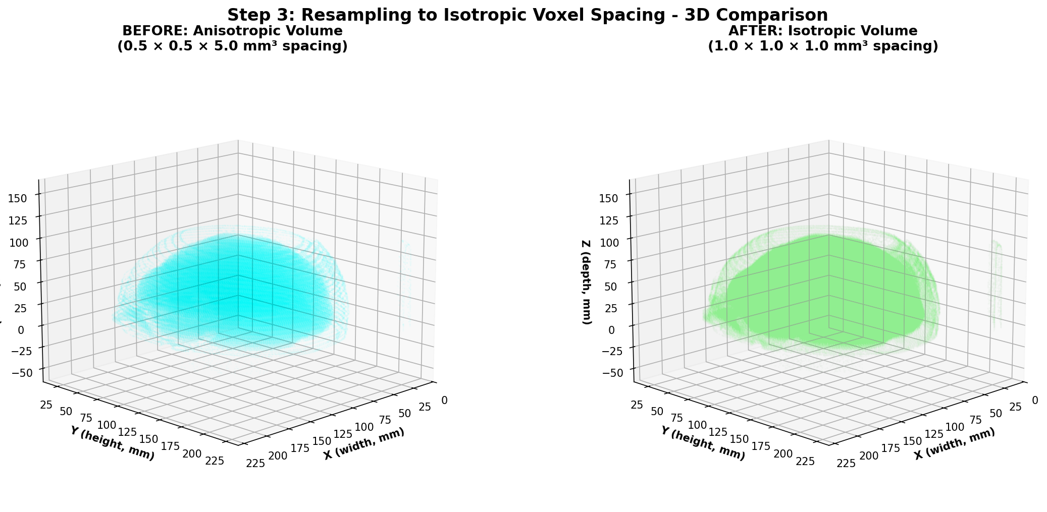
One thing to note about medical imaging data is that the spacing between slices (z-axis) can vary significantly between different scans due to differences in acquisition protocols or patient positioning especially when combining different datasets. This is also the case for the in-plane resolution (x and y axes) denoted by the PixelSpacing DICOM field. Additionally, within the same scan, the spacing along the z-axis can also differ between slices in some cases. This variability can pose challenges when training deep learning models, especially 3D convolutional neural networks (CNNs), as they require consistent spatial resolution across all input volumes. To address this issue, resampling the volume to a standard voxel size is a common preprocessing step as this makes each input volume have the same voxel spacing. To be clear, a voxel is the 3D equivalent of a pixel, representing a value on a regular grid in three-dimensional space and voxel spacing refers to the physical distance between the centers of adjacent voxels along each axis (x, y, z) with each value along one axis being generally in millimeters for CT scans applications.

Conceptually, the original volume is a sampled version of a continuous underlying density function. Resampling changes the sampling grid: we replace the original 3D grid with a new 3D grid that has the target spacing. The image intensities at new grid points are computed by interpolation from the old grid. After resampling, the image still represents the same physical volume, but sampled at a different resolution that will be uniform meaning the same for all the voxels on the grid and across different scans.

Different interpolation methods can be chosen for resampling. The one thing to keep in mind is that when choosing the right method, it is mostly about finding a sweet spot between computational efficiency and image quality preservation. The most common methods are:

NearestNeighbor that is used for label maps and segmentation masks. This method assigns for each voxel on the new grid the value of the closest original voxel. It is simple and preserves the discrete nature of labels that should not be interpolated.
Trilinear interpolation uses 8 neighboring known-voxels (a cube) to interpolate a weighted average based on fractional distances along x,y,z. It is fast and provides reasonably smooth results, making it a popular choice for medical images.
Cubic Interpolation uses 64 neighboring voxels to fit a cubic polynomial along each axis, providing smoother results than trilinear interpolation. It is more computationally intensive but can better preserve image details.
B-Spline Interpolation is based on fitting piecewise polynomial functions (B-splines) to the data. It can provide very smooth results and is good at preserving image features, but is also computationally demanding like cubic interpolation.

Finally, one thing we did not talk about yet is the choice of the target voxel size which will determine the new 3D grid of points. This choice is often empirical and based on the spacing values of your dataset. One could for example choose an isotropic voxel size of 1x1x1 mm³ if the original spacing values are close to that. Intuitively, a smaller voxel size will preserve more details but increase computational cost and memory usage, while a larger voxel size will reduce detail but be more efficient. Moreover, having a voxel size that allows the voxels on the new grid to be close to one original voxel is a good idea to avoid interpolating too much and thus losing information.

By the way, when resampling, do not forget to apply the same transformation to any associated segmentation masks or label maps using NearestNeighbor interpolation to ensure alignment with the resampled image. This also goes for all other operations on the whole volumes like slice ordering, or data augmentations operations.

Let's implement a Linear resampling function in Python using SciPy module. Note that using SimpleITK or other medical imaging libraries is sometimes a good idea as they have optimized functions for that purpose but if your scan volumes do not have a uniform spacing, SimpleITK will enforce you to resample the volume to a uniform spacing to have a SimpleITK Image before even applying any transformations which can lead to 2 consecutives resampling and more artifacts or loss of information.

def resample_isotropic_scipy(
    volume: np.ndarray,
    z_positions: np.ndarray,
    target_spacing: Tuple[float, float, float],
) -> Tuple[np.ndarray, np.ndarray]:

    dx, dy = volume[0].PixelSpacing # assuming uniform spacing in the slice plane
    tx, ty, tz = target_spacing
    y = np.arange(volume.shape[1]) * dy
    x = np.arange(volume.shape[2]) * dx
    y_new = np.arange(0, y[-1] + 1e-4, ty)
    x_new = np.arange(0, x[-1] + 1e-4, tx)
    z_new = np.arange(z_positions[0], z_positions[-1] + 1e-4, tz)
    interpolator = interpolate.RegularGridInterpolator(
        (z_positions, y, x), volume, bounds_error=False, fill_value=-1000
    ) # fill_value for areas outside original volume, usually air in CT scans so -1000 HU
    zz, yy, xx = np.meshgrid(z_new, y_new, x_new, indexing="ij") # create new grid of points

  new_grid = np.stack([zz.ravel(), yy.ravel(), xx.ravel()], axis=-1)

  resampled = interpolator(new_grid).reshape(len(z_new), len(y_new), len(x_new))
    return resampled.astype(np.float32), z_new.astype(np.float32)

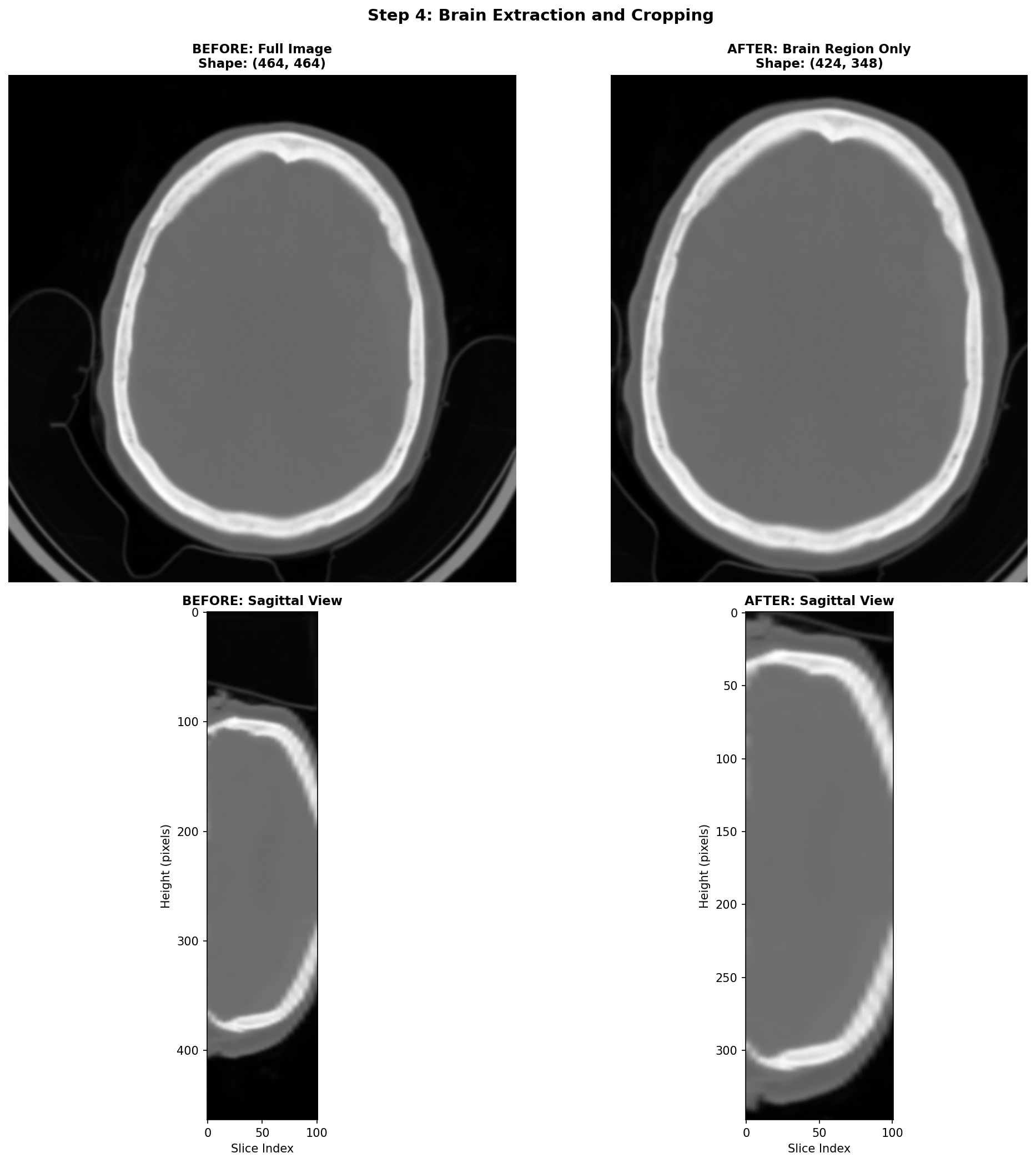
4) Brain Extraction and Cropping Techniques

When working with CT head scans, the images dealt with often are images that include not just the brain, but also the skull, scalp, neck tissues, and sometimes even scanner table or artefacts on the edges. For stroke detection, most of this extra information is irrelevant noise that can confuse our deep learning models and slow down training.

The most practical starting point for brain cropping leverages a fundamental property of CT imaging: brain tissue has a predictable range of intensity values. We can create a binary mask by simply keeping everything in the brain tissue range, and casting away the rest.

This simple approach is fast and can be effective for most stroke detection applications. Its main limitation is that it doesn't produce a true brain mask, it just finds a tight bounding box around brain-intensity tissues. If the need to use more sophisticated brain extraction methods arises, there are deep learning models like SynthStrip or the method by Liu et al. that can generate accurate brain masks. However, these methods require additional dependencies and computational resources, so they should be used only if the simple thresholding approach proves inadequate.

An important remark is that this step can be skipped if your application requires a fixed sized input size for your model, and so cropping the brain region and then padding to a fixed size is sometimes just equivalent to skipping this step and directly resizing the whole volume to the fixed size. As a general rule, always visualize the data through the whole processing pipeline to tailor it the best way possible to your specific task.

Here's how this works step-by-step:

Create the mask: Keep only voxels with HU values in the brain range
Select the brain: Use connected component analysis to keep only the largest connected region (the brain)
Find the bounding box: Determine the smallest rectangular volume that contains all brain voxels
Add margin: Expand the box slightly to avoid cutting off edge structures

def crop_brain_simple(volume: np.ndarray, hu_range: Tuple[int, int] = (-200, 500)) -> Tuple[np.ndarray, Tuple[slice, slice, slice]]:
    """
    Crop brain volume using simple intensity thresholding.

    Args:
        volume: 3D numpy array in Hounsfield Units
        hu_range: Tuple of (min_hu, max_hu) for brain tissue

    Returns:
        Cropped volume and the slice indices used for cropping
    """
    from scipy import ndimage

    # Step 1: Create binary mask for brain tissue
    brain_mask = (volume >= hu_range[0]) & (volume <= hu_range[1])

    # Step 2: Remove small disconnected components, keep largest (brain)
    labeled, num_features = ndimage.label(brain_mask)
    if num_features > 1:
        sizes = ndimage.sum(brain_mask, labeled, range(num_features + 1))
        brain_mask = sizes[labeled] == sizes.max()

    # Step 3: Find bounding box coordinates
    coords = np.array(np.where(brain_mask))
    z_min, y_min, x_min = coords.min(axis=1)
    z_max, y_max, x_max = coords.max(axis=1)

    # Step 4: Add margin to avoid cutting edge structures
    margin = 2
    z_slice = slice(max(0, z_min - margin), min(volume.shape[0], z_max + margin + 1))
    y_slice = slice(max(0, y_min - margin), min(volume.shape[1], y_max + margin + 1))
    x_slice = slice(max(0, x_min - margin), min(volume.shape[2], x_max + margin + 1))

    cropped = volume[z_slice, y_slice, x_slice]
    return cropped, (z_slice, y_slice, x_slice)

Here, the brain cropping operation mainly removes artefacts related to the scanner table and some neck tissues.

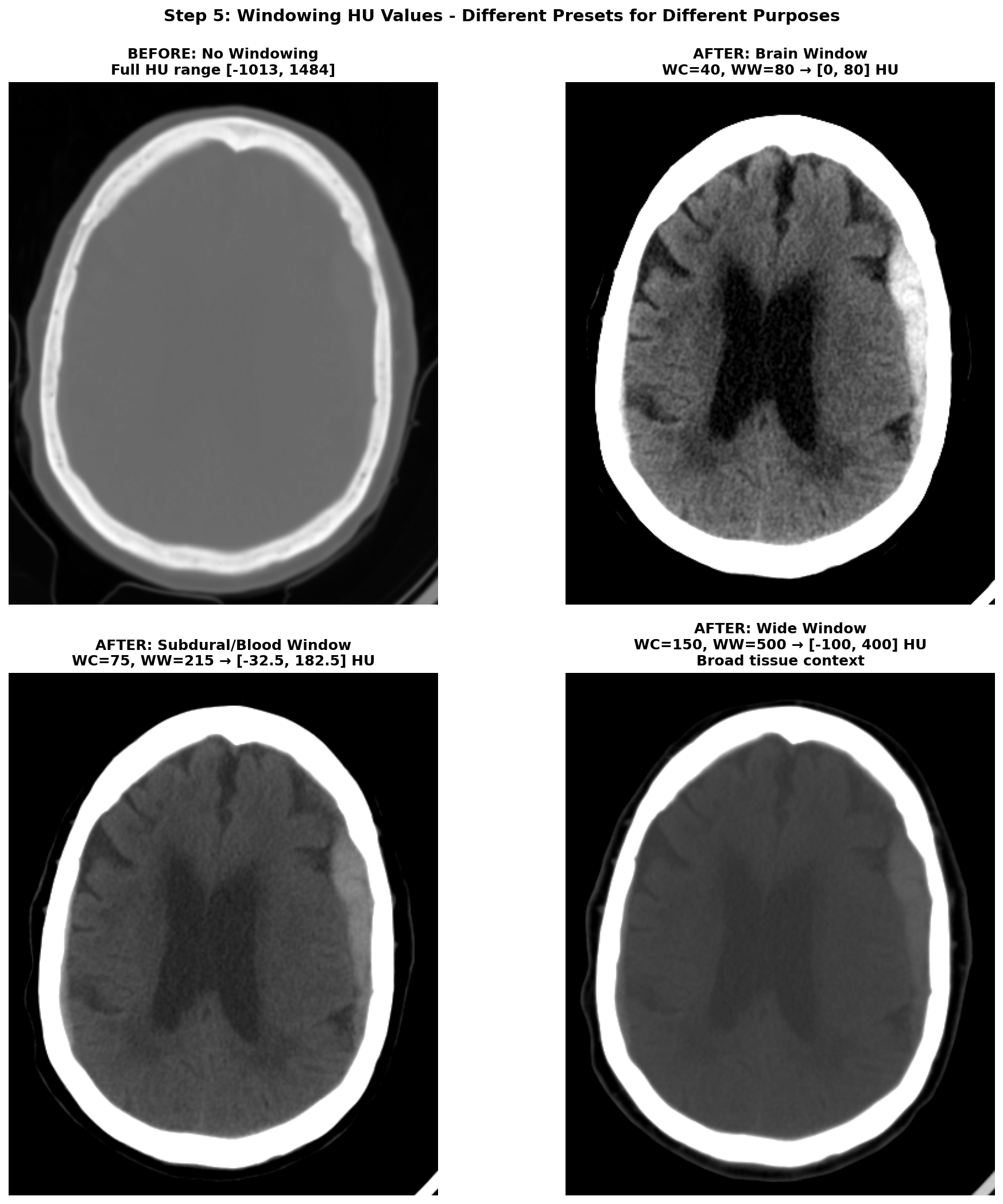
5) Windowing the range of Hounsfield Units (HU)

The HU scale is quite wide, ranging from -1000 HU for air to more than +1000 HU for dense bone. And in this wide range of value, only a small subset is really useful for brain CT scans analysis. The rest of the non-useful information can be considered as noise that can make the learning task harder for a deep learning model. Hence the need to restrict the range of HU values. This is achieved through a technique called windowing in medical imaging. Windowing involves selecting a range of Housefield Units values judged pertinent for the task at hand and remapping all values outside this range to the closest extremum of the range. The range is commonly defined by giving a window center (WC or WL) and a window width (WW). The range of HU values is then $[WC - WW/2, WC + WW/2]$ .

There are several standard window settings for different tissues and pathologies. The exact value can vary slightly between studies and articles but the most common ones for deep learning applications are:

Brain window (parenchyma) — WC = 40, WW = 80 → HU range [0, 80] This is the standard brain window used clinically for evaluating brain tissues.
Subdural / blood window — WC = 75, WW = 215 → HU range [-32.5, 182.5] (some studies also use WL 50-100, WW 130-300 for thin subdural detection). This enhances acute blood detection and thin subdural hematomas, providing better contrast for hemorrhagic pathology.
Wide / raw window — [-100, 400] → preserves broad context including edema and most pathologic ranges while suppressing bone and air artifacts. This provides comprehensive tissue visualization without losing important diagnostic information.

Narrow windows (very small WW) are generally poor choices because they can amplify scanner noise so are a bit risky to use for deep learning applications.

After applying windowing to restrict the HU range, the data typically needs to be scaled for optimal neural network training. The most common scaling approach is a min-max normalization to [0, 1] range:

$scaled = (WindowedImage - Wmin) / (Wmax - Wmin)$ with $Wmin$ and $Wmax$ being the minimum and maximum HU values of the chosen window.

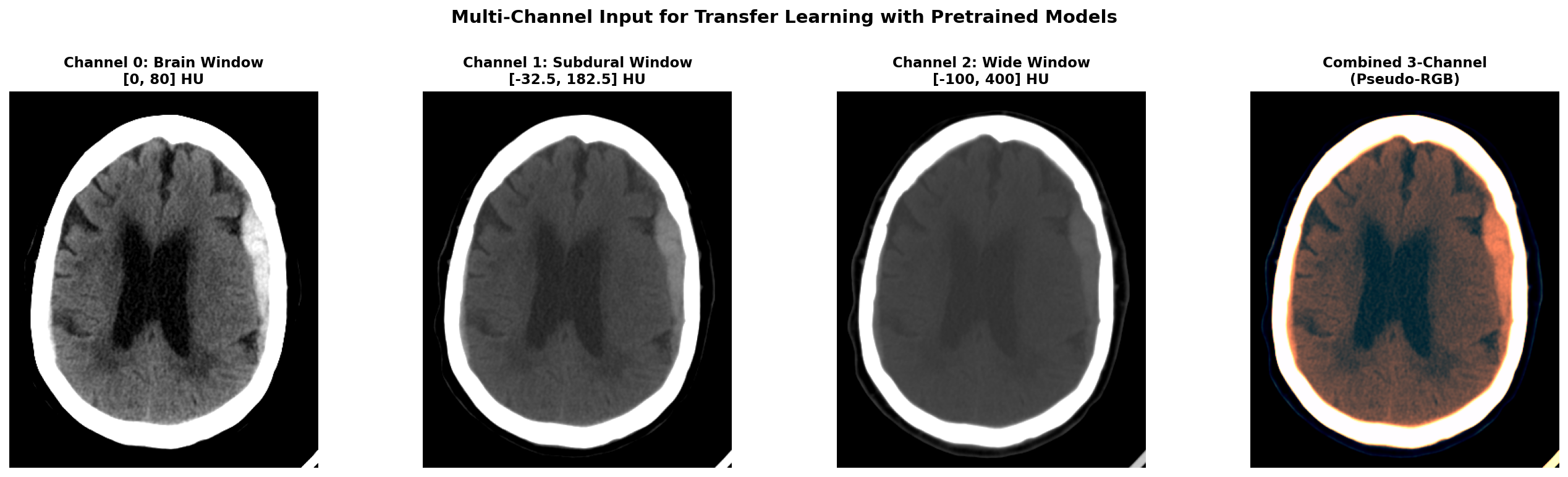
Applying multiple window settings to get multiple channels of input data can be a great idea to provide different level of information to the model. It can also be useful when leveraging pretrained 2D models that expect 3-channel input like RGB images. In this case, you can create a 3-channel input where each channel corresponds to a different window setting (e.g., brain window, subdural window, wide window). This way, you can utilize the rich information from multiple windows while still benefiting from transfer learning with pretrained models.

Here is a Python code snippet to illustrate the windowing and scaling process applied on a single 2D slice:

def apply_windowing(self, img, center, width):
    """Apply CT windowing based on preset"""
    image = img.copy()
    min_value = center - width // 2
    max_value = center + width // 2
    image = np.clip(image, min_value, max_value)
    img_normalized = (image - min_value) / width
    return img_normalized

The effect of windowing is demonstrated below on our RSNA hemorrhagic stroke case. The left panel shows the full HU range (-1000 to +1000 HU) where bone appears very bright, making it difficult to distinguish subtle brain tissue variations. The middle panel applies the standard brain window (WC=40, WW=80, range [0, 80] HU), which optimally displays brain parenchyma and clearly highlights the hemorrhagic region as a bright hyperintense area. The right panel shows the subdural/blood window (WC=75, WW=215, range [-32.5, 182.5] HU), which is specifically designed to enhance blood detection and provides excellent contrast for the hemorrhage while still showing surrounding brain tissue.

When applying multiple windows to create multi-channel input (for example when using pretrained models expecting RGB input), here's what the different channels look like. Below we show our hemorrhagic stroke case with three different window settings applied simultaneously.

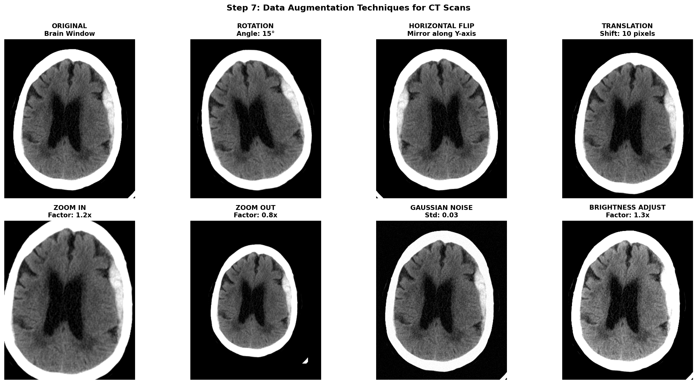
6) Data augmentation techniques for CT scans

Once all the previous preprocessing steps are complete, data augmentation becomes a powerful tool to artificially increase the size and diversity of your training dataset. This is especially crucial in medical imaging where datasets are often small, expensive to acquire, and imbalanced between normal and pathological cases. However, unlike natural images where aggressive augmentations are common, medical images require careful consideration to maintain clinical validity and avoid creating anatomically impossible or diagnostically misleading examples.

The golden rule for medical image augmentation is that transformed images must remain clinically plausible. A brain CT scan can be horizontally flipped because stroke pathology can occur on either hemisphere, but vertical flipping would be nonsensical. Similarly, slight rotations account for patient positioning variations, but extreme rotations would create unrealistic orientations never seen in clinical practice.

Augmentations are meant to simulate natural variations in patient positioning, scanner differences, and acquisition protocols. Horizontal flipping mirrors the image left-to-right which can be applied for stroke detection because a stroke can be present in both hemispheres while maintaining anatomical validity. Translations can account for slight positioning variations but it can also remove a part of the brain tissues. Small Rotations can also improve robustness by simulating patient positioning differences during exam acquisition but it shifts the pixel from the original grid and thus requires interpolation. Affine transformations can simulate slight scaling or shearing due to different head sizes or scanner distortions but should be kept minimal to avoid unrealistic deformations. Intensity transformations can also be useful to simulate light scanner noise: adding Gaussian noise, and applying slight brightness contrast adjustments by stretching or shifting the intensity values.

To implement these augmentations, MONAI is a great library specifically designed for medical imaging that provides a wide range of 2D and 3D augmentations with support for both images and segmentation masks. Transformation function can be found in the module monai.transforms with for example RandFlip, RandRotate, RandAffine, RandGaussianNoise, and RandAdjustContrast corresponding to the augmentations described above.

Notice that spatial transforms must be applied to both the image and mask with identical parameters, while intensity transforms are only applied to the image since masks contain discrete labels that shouldn't be interpolated or have noise added.

This should go without saying, but augmentation should only be applied during training. Validation and test sets must use the original, unaugmented images to provide honest performance estimates. The validation transforms should only include necessary preprocessing steps (HU conversion, resampling, windowing).

To help visualize the effect of augmentations, here are some examples applied to our hemorrhagic stroke case:

D) Concluding remarks

And we are finally done! We've journeyed through the complete CT preprocessing pipeline, from understanding DICOM's data format to having a processed and ready to use dataset for deep learning applications.

The most important lesson? Always tailor these steps to your data at each processing stage. Visualization and implementing small sanity checks are key. This can save a lot of time as an entire pipeline can be computationally quite expensive if run on a consequent dataset. I remember ignoring at first my own advice and ended up having to find a needle in a haystack in a faulty processing pipeline — which was just improper stacking of my 2D mask slices that was off from the image slices!
Anyway, I hope this guide has provided useful insights on how to approach processing CT images for deep learning applications. If you are curious about the next steps after preprocessing, stay tuned for future posts where we will explore model architectures, training strategies, and evaluation metrics specifically tailored for stroke detection tasks.

References

[1] Partial Encryption Scheme of Medical Images Based on DWT, Secret Image Sharing and Hyperchaotic System - Scientific Figure on ResearchGate. Available from: https://www.researchgate.net/figure/The-three-perspective-planes-used-in-medical-imaging-are-Axial-or-Transversal-Coronal_fig1_383827964
[2] Barthels, D., & Das, H. (2020). Current advances in ischemic stroke research and therapies. Biochimica et Biophysica Acta (BBA) - Molecular Basis of Disease, 1866(4), 165260. https://pmc.ncbi.nlm.nih.gov/articles/PMC11786524/pdf/10.1177_17474930241308142.pdf
[3] https://www.dicomstandard.org/about
[4] PyDicom Development Team. (2023). PyDicom Documentation. Retrieved from https://pydicom.github.io/
[5] Radiopaedia.org. "Windowing (CT)." Retrieved from https://radiopaedia.org/articles/windowing-ct
[6] Liu, X., Feng, Z., Wu, Y., et al. (2023). A fast and accurate brain extraction method for CT head images. BMC Medical Imaging, 23, 147. https://bmcmedimaging.biomedcentral.com/articles/10.1186/s12880-023-01097-0
[7] Hoopes, A., Mora, J. S., Dalca, A. V., Fischl, B., & Hoffmann, M. (2022). SynthStrip: skull-stripping for any brain image. NeuroImage, 260, 119474. https://pmc.ncbi.nlm.nih.gov/articles/PMC9465771/
[8] Anjali Gautam, Balasubramanian Raman, Towards effective classification of brain hemorrhagic and ischemic stroke using CNN, Biomedical Signal Processing and Control, Volume 63, 2021, 102178, ISSN 1746-8094, https://doi.org/10.1016/j.bspc.2020.102178.