Building a Reproducible Multimodal Pipeline

This article is the second in a series of posts where I share my journey exploring proteomics, cancer biology, and AI-driven solutions for oncology. In the upcoming posts, I will expand on the data foundations of the project, the machine learning methods we are testing, and the clinical implications of this research. The goal of the series is to make complex concepts accessible while also showing the step-by-step progress of building an applied research project from biology to artificial intelligence. Stay tuned if you are curious about how molecular data, medical images, and deep learning can come together to address one of the most fundamental challenges in cancer research.

---

How to pair RNA-seq data with WSI data?

In Post 1 we asked: can H&E histology carry a footprint of telomerase activity? Here we operationalize that idea: assemble images and RNA for the same patients, create a robust telomerase-high label, and produce clean tensors for modeling.

Several public resources exist (e.g., TCGA = The Cancer Genome Atlas; CPTAC = Clinical Proteomic Tumor Analysis Consortium). We use TCGA because it provides, at population scale, paired WSIs + RNA-seq, harmonized pipelines, rich metadata, and open GCS access via ISB-CGC (Institute for Systems Biology - Cancer Genomics Cloud, an NCI-funded platform). That makes it ideal for reproducible ETL.

TCGA assigns every specimen a structured barcode. An example is shown in Figure 1. The components we care about first are:

• Project: The program name (e.g., TCGA or CPTAC).
• TSS (Tissue Source Site): The collection center code (e.g., “02” for MD Anderson).
• Participant: An alphanumeric patient identifier.
• Sample: The sample type (e.g., “01” = primary solid tumor; “11” = solid tissue normal; tumor types 01–09, normals 10–19, controls 20–29).
• Vial: A letter A–Z indicating the vial/order.

Using the structured barcode, we can join data reliably. For labels computed at the patient level, we attach RNA to slides via the case barcode (TCGA-XX-YYYY). When we need stricter pairing at the sample level, we use the sample barcode (first five components). Following this procedure, more than 10k samples were paired.

Pulling data from BigQuery (ISB-CGC)

BigQuery is Google Cloud’s serverless, scalable data warehouse where you can run super fast SQL analytics on massive datasets without managing infrastructure. Through ISB-CGC, it hosts TCGA tables we need:

• RNA-seq: isb-cgc-bq.TCGA_versioned.RNAseq_hg38_gdc_r42

  • We focus on TERT (telomerase reverse transcriptase), the catalytic subunit of telomerase that adds TTAGGG repeats to telomeres using the TERC RNA template (see Post 1).
  • We use tpm_unstranded (transcripts per million; library-size–normalized expression) to build the telomerase-high label.

• Slides: isb-cgc-bq.TCGA.slide_images_gdc_current

  • We read file_gcs_url (GCS path to the WSI) and AppMag (acquisition magnification, useful for consistent patch scale).

If you like pandas-style queries, ibis lets you write SQL as Python expressions and read directly to DataFrames.

import ibis # SQL as pandas
import pandas as pd

OUT_BUCKET= "gs://processed_data"

con = ibis.bigquery.connect(project_id='project-id')


# Import RNA-seq data
rna_table = con.table('isb-cgc-bq.TCGA_versioned.RNAseq_hg38_gdc_r42')

filtered_rna = (rna_table
                .filter(rna_table.gene_name=='TERT')
                .select('project_short_name', 'case_barcode', 'sample_barcode', 'gene_name', 'tpm_unstranded')
                .pivot_wider(names_from="gene_name", values_from="tpm_unstranded")
                )

df_rna = filtered_rna.execute()


# import WSI data
wsi_table = con.table('isb-cgc-bq.TCGA.slide_images_gdc_current')
filtered_wsi = (wsi_table
                .select('sample_barcode', 'slide_barcode', 'svsFilename','file_gcs_url','AppMag')
                )

df_wsi = filtered_wsi.execute()

# Merge RNA-seq and WSI data on sample_barcode
df_merged = (
    df_rna[['project_short_name', 'case_barcode', 'sample_barcode']]
    .merge(df_wsi, on='sample_barcode', how='inner')
    .sort_values(by=['project_short_name','case_barcode'])
)

Finally, across cohorts we compute the 75th percentile (Q3) of TERT expression and define the labels:

• Label = 1: TERT ≥ Q3 (telomerase-high)
• Label = 0: otherwise

In plain terms: a slide is considered telomerase-high if its TERT reading falls in the top quartile.

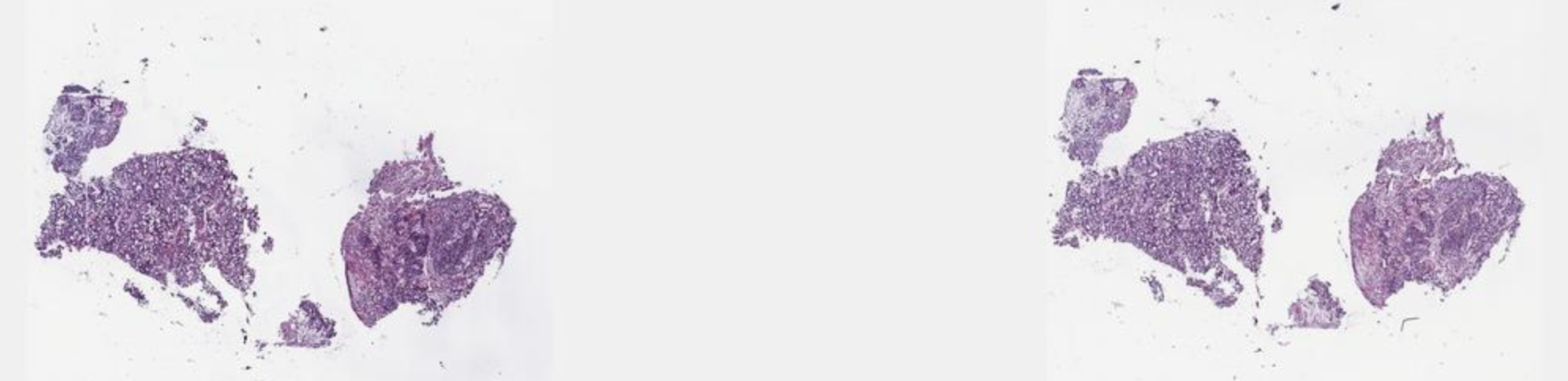
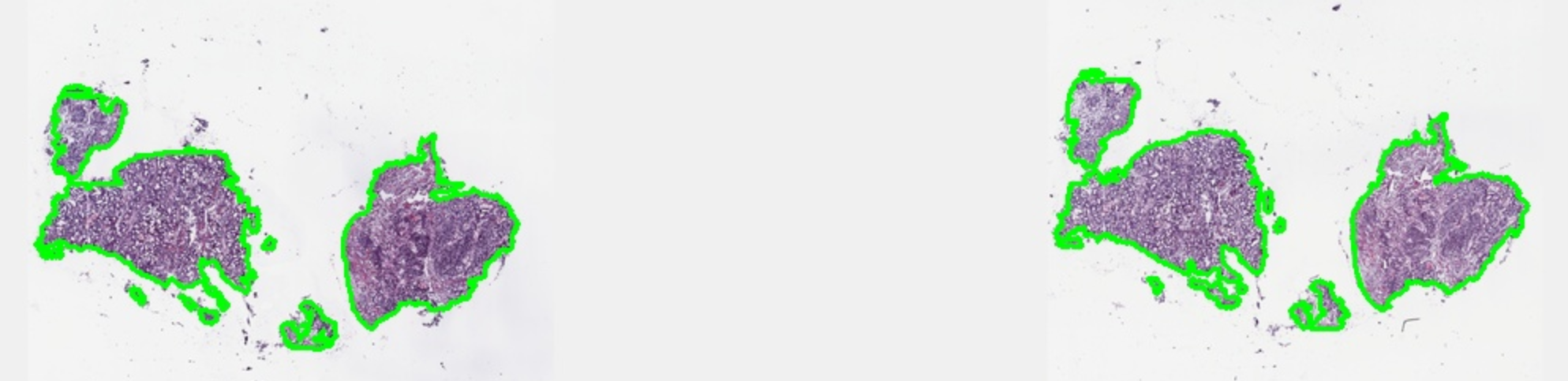
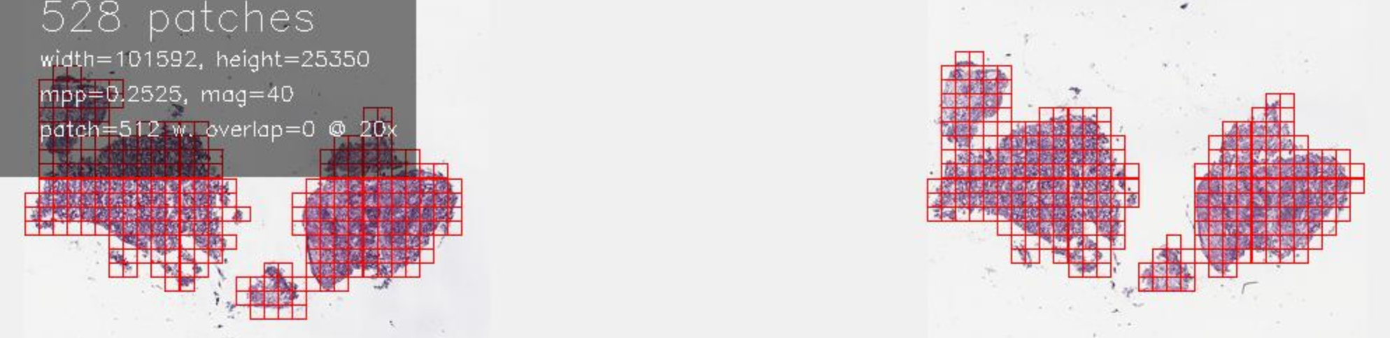
Patch embeddings of WSI

Whole-slide images (WSIs) are huge, high-resolution images. To get local representations, we (1) detect tissue, (2) tile it into smaller patches, and (3) compute patch embeddings with a vision transformer. The TRIDENT library can run this end-to-end in one command:

python trident/run_batch_of_slides.py --task all \
  --wsi_dir path_to_slide_images \
  --job_dir path_to_outputs \
  --patch_encoder uni_v2 \
  --mag 20 \
  --patch_size 256 \
  --remove_artifacts \
  --max_workers 8

Other patch encoders besides uni_v2 are available (see the TRIDENT repo). The patch_size and embedding dimensionality depend on the chosen encoder, so pick accordingly. Some WSIs contain pen marks or artifacts; --remove_artifacts helps filter them.

Embeddings are written under path_to_outputs as one .h5 file per slide, containing an array of shape (num_patches, embedding_dim) plus patch coordinates. With uni_v2, the embedding dimension is 1536; the number of patches varies per slide. Computing embeddings is time-consuming; an alternative is the precomputed UNI2-h features on Hugging Face. If you use those, pairing with RNA-seq requires two merges:

1. precomputed embeddings and WSI table on slide_barcode, then
2. that result and RNA-seq on case_barcode.

At this point, each WSI is represented by many patch embeddings, while TERT gives one label per slide. Intuitively, only a subset of patches drives the telomerase signal.

A baseline classifier on pooled image features

We conclude with a simple baseline: compute a slide embedding as the mean of its patch embeddings, then feed it to a small MLP (see BaselineClassifier below).

This “mean-pool + MLP” setup is clean and reproducible, and it confirms that an image-only signal correlates with telomerase (see Figure 4). In Post 3, we’ll replace mean pooling with Attention-based Multi-Instance Learning (ABMIL) to generate patch-level heatmaps that localize the signal on WSIs.

class BaselineClassifier(nn.Module):
    def __init__(self, img_dim=1536, p=0.2):
        super().__init__()
        self.img_fc1 = nn.Linear(img_dim, 1024, bias=False)
        self.img_post = nn.Sequential(
            nn.GELU(), nn.Dropout(p),
            nn.Linear(1024, 512), nn.GELU(), nn.Dropout(p)
        )
        self.res = nn.Sequential(
            nn.Linear(512, 512), nn.GELU(), nn.Dropout(p),
            nn.Linear(512, 512)
        )
        self.head = nn.Sequential(
            nn.Linear(512, 256), nn.GELU(), nn.Dropout(p),
            nn.Linear(256, 1)
        )
    def forward(self, x_img):
        z = self.img_post(self.img_fc1(x_img))
        z = z + self.res(z)
        return self.head(z).squeeze(1)